Clustering

Claus O. Wilke

2025-03-21

 

These points correspond to three clusters. Can a computer find them automatically?

 

These points correspond to three clusters. Can a computer find them automatically?

k-means clustering

1. Start with k randomly chosen means

2. Color data points by the shortest distance to any mean

3. Move means to centroid position of each group of points

4. Repeat from step 2 until convergence

Let’s try it out

 

 

Add means at arbitrary locations

 

Color data points by the shortest distance to any mean

 

Color data points by the shortest distance to any mean

 

Move means to centroid position of each group of points

 

Color data points by the shortest distance to any mean

 

Color data points by the shortest distance to any mean

 

Move means to centroid position of each group of points

 

Color data points by the shortest distance to any mean

 

Color data points by the shortest distance to any mean

 

Move means to centroid position of each group of points

 

Color data points by the shortest distance to any mean

 

Color data points by the shortest distance to any mean

 

Move means to centroid position of each group of points

 

Color data points by the shortest distance to any mean

 

Color data points by the shortest distance to any mean

 

Move means to centroid position of each group of points

 

Color data points by the shortest distance to any mean

 

Color data points by the shortest distance to any mean

 

Final result

Now we’ll cluster the same dataset with five centroids

 

 

Add means at arbitrary locations

 

Color data points by the shortest distance to any mean

 

Color data points by the shortest distance to any mean

 

Move means to centroid position of each group of points

 

Color data points by the shortest distance to any mean

 

Color data points by the shortest distance to any mean

 

Move means to centroid position of each group of points

 

Color data points by the shortest distance to any mean

 

Color data points by the shortest distance to any mean

 

Move means to centroid position of each group of points

 

Color data points by the shortest distance to any mean

 

Color data points by the shortest distance to any mean

 

Move means to centroid position of each group of points

 

Color data points by the shortest distance to any mean

 

Color data points by the shortest distance to any mean

 

Move means to centroid position of each group of points

… do many more iterations …

 

Final result

Now let’s try the spirals dataset

 

 

Add means at arbitrary locations

 

Color data points by the shortest distance to any mean

 

Color data points by the shortest distance to any mean

 

Move means to centroid position of each group of points

 

Color data points by the shortest distance to any mean

 

Color data points by the shortest distance to any mean

 

Move means to centroid position of each group of points

 

Color data points by the shortest distance to any mean

 

Color data points by the shortest distance to any mean

 

Move means to centroid position of each group of points

 

Color data points by the shortest distance to any mean

 

Color data points by the shortest distance to any mean

 

Move means to centroid position of each group of points

 

Color data points by the shortest distance to any mean

 

Color data points by the shortest distance to any mean

 

Move means to centroid position of each group of points

… do many more iterations …

 

Final result

k-means clustering works best when
data forms distinct, compact clusters

Other clustering algorithms

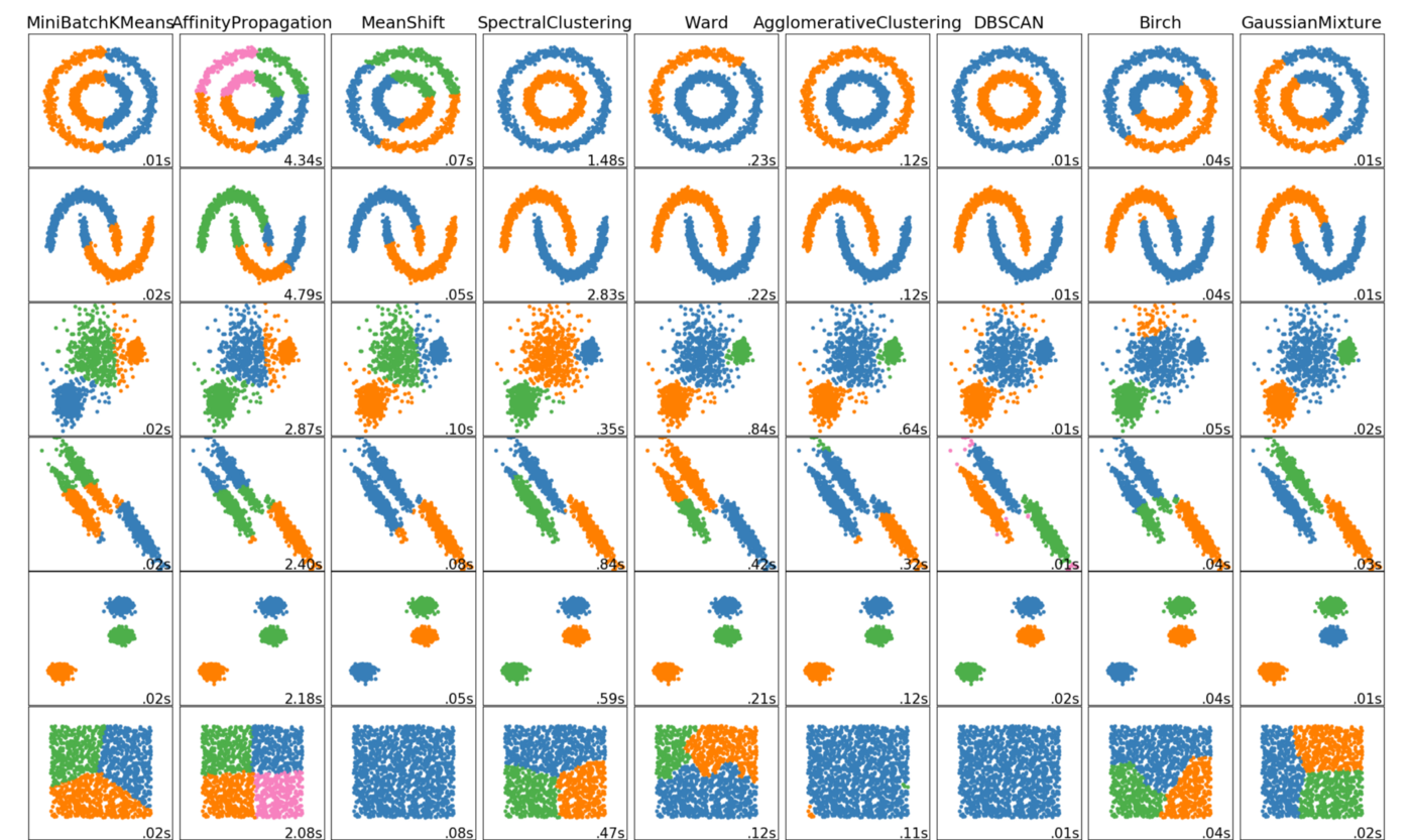
From George Seif (2018) The 5 Clustering Algorithms Data Scientists Need to Know

Doing k-means clustering in R

Example dataset: iris

Measurements on the sepals and petals of three iris species

iris

    Sepal.Length Sepal.Width Petal.Length Petal.Width    Species
1            5.1         3.5          1.4         0.2     setosa
2            4.9         3.0          1.4         0.2     setosa
3            4.7         3.2          1.3         0.2     setosa
4            4.6         3.1          1.5         0.2     setosa
5            5.0         3.6          1.4         0.2     setosa
6            5.4         3.9          1.7         0.4     setosa
7            4.6         3.4          1.4         0.3     setosa
8            5.0         3.4          1.5         0.2     setosa
9            4.4         2.9          1.4         0.2     setosa
10           4.9         3.1          1.5         0.1     setosa
11           5.4         3.7          1.5         0.2     setosa
12           4.8         3.4          1.6         0.2     setosa
13           4.8         3.0          1.4         0.1     setosa
14           4.3         3.0          1.1         0.1     setosa
15           5.8         4.0          1.2         0.2     setosa
16           5.7         4.4          1.5         0.4     setosa
17           5.4         3.9          1.3         0.4     setosa
18           5.1         3.5          1.4         0.3     setosa
19           5.7         3.8          1.7         0.3     setosa
20           5.1         3.8          1.5         0.3     setosa
21           5.4         3.4          1.7         0.2     setosa
22           5.1         3.7          1.5         0.4     setosa
23           4.6         3.6          1.0         0.2     setosa
24           5.1         3.3          1.7         0.5     setosa
25           4.8         3.4          1.9         0.2     setosa
26           5.0         3.0          1.6         0.2     setosa
27           5.0         3.4          1.6         0.4     setosa
28           5.2         3.5          1.5         0.2     setosa
29           5.2         3.4          1.4         0.2     setosa
30           4.7         3.2          1.6         0.2     setosa
31           4.8         3.1          1.6         0.2     setosa
32           5.4         3.4          1.5         0.4     setosa
33           5.2         4.1          1.5         0.1     setosa
34           5.5         4.2          1.4         0.2     setosa
35           4.9         3.1          1.5         0.2     setosa
36           5.0         3.2          1.2         0.2     setosa
37           5.5         3.5          1.3         0.2     setosa
38           4.9         3.6          1.4         0.1     setosa
39           4.4         3.0          1.3         0.2     setosa
40           5.1         3.4          1.5         0.2     setosa
41           5.0         3.5          1.3         0.3     setosa
42           4.5         2.3          1.3         0.3     setosa
43           4.4         3.2          1.3         0.2     setosa
44           5.0         3.5          1.6         0.6     setosa
45           5.1         3.8          1.9         0.4     setosa
46           4.8         3.0          1.4         0.3     setosa
47           5.1         3.8          1.6         0.2     setosa
48           4.6         3.2          1.4         0.2     setosa
49           5.3         3.7          1.5         0.2     setosa
50           5.0         3.3          1.4         0.2     setosa
51           7.0         3.2          4.7         1.4 versicolor
52           6.4         3.2          4.5         1.5 versicolor
53           6.9         3.1          4.9         1.5 versicolor
54           5.5         2.3          4.0         1.3 versicolor
55           6.5         2.8          4.6         1.5 versicolor
56           5.7         2.8          4.5         1.3 versicolor
57           6.3         3.3          4.7         1.6 versicolor
58           4.9         2.4          3.3         1.0 versicolor
59           6.6         2.9          4.6         1.3 versicolor
60           5.2         2.7          3.9         1.4 versicolor
61           5.0         2.0          3.5         1.0 versicolor
62           5.9         3.0          4.2         1.5 versicolor
63           6.0         2.2          4.0         1.0 versicolor
64           6.1         2.9          4.7         1.4 versicolor
65           5.6         2.9          3.6         1.3 versicolor
66           6.7         3.1          4.4         1.4 versicolor
67           5.6         3.0          4.5         1.5 versicolor
68           5.8         2.7          4.1         1.0 versicolor
69           6.2         2.2          4.5         1.5 versicolor
70           5.6         2.5          3.9         1.1 versicolor
71           5.9         3.2          4.8         1.8 versicolor
72           6.1         2.8          4.0         1.3 versicolor
73           6.3         2.5          4.9         1.5 versicolor
74           6.1         2.8          4.7         1.2 versicolor
75           6.4         2.9          4.3         1.3 versicolor
76           6.6         3.0          4.4         1.4 versicolor
77           6.8         2.8          4.8         1.4 versicolor
78           6.7         3.0          5.0         1.7 versicolor
79           6.0         2.9          4.5         1.5 versicolor
80           5.7         2.6          3.5         1.0 versicolor
81           5.5         2.4          3.8         1.1 versicolor
82           5.5         2.4          3.7         1.0 versicolor
83           5.8         2.7          3.9         1.2 versicolor
84           6.0         2.7          5.1         1.6 versicolor
85           5.4         3.0          4.5         1.5 versicolor
86           6.0         3.4          4.5         1.6 versicolor
87           6.7         3.1          4.7         1.5 versicolor
88           6.3         2.3          4.4         1.3 versicolor
89           5.6         3.0          4.1         1.3 versicolor
90           5.5         2.5          4.0         1.3 versicolor
91           5.5         2.6          4.4         1.2 versicolor
92           6.1         3.0          4.6         1.4 versicolor
93           5.8         2.6          4.0         1.2 versicolor
94           5.0         2.3          3.3         1.0 versicolor
95           5.6         2.7          4.2         1.3 versicolor
96           5.7         3.0          4.2         1.2 versicolor
97           5.7         2.9          4.2         1.3 versicolor
98           6.2         2.9          4.3         1.3 versicolor
99           5.1         2.5          3.0         1.1 versicolor
100          5.7         2.8          4.1         1.3 versicolor
101          6.3         3.3          6.0         2.5  virginica
102          5.8         2.7          5.1         1.9  virginica
103          7.1         3.0          5.9         2.1  virginica
104          6.3         2.9          5.6         1.8  virginica
105          6.5         3.0          5.8         2.2  virginica
106          7.6         3.0          6.6         2.1  virginica
107          4.9         2.5          4.5         1.7  virginica
108          7.3         2.9          6.3         1.8  virginica
109          6.7         2.5          5.8         1.8  virginica
110          7.2         3.6          6.1         2.5  virginica
111          6.5         3.2          5.1         2.0  virginica
112          6.4         2.7          5.3         1.9  virginica
113          6.8         3.0          5.5         2.1  virginica
114          5.7         2.5          5.0         2.0  virginica
115          5.8         2.8          5.1         2.4  virginica
116          6.4         3.2          5.3         2.3  virginica
117          6.5         3.0          5.5         1.8  virginica
118          7.7         3.8          6.7         2.2  virginica
119          7.7         2.6          6.9         2.3  virginica
120          6.0         2.2          5.0         1.5  virginica
121          6.9         3.2          5.7         2.3  virginica
122          5.6         2.8          4.9         2.0  virginica
123          7.7         2.8          6.7         2.0  virginica
124          6.3         2.7          4.9         1.8  virginica
125          6.7         3.3          5.7         2.1  virginica
126          7.2         3.2          6.0         1.8  virginica
127          6.2         2.8          4.8         1.8  virginica
128          6.1         3.0          4.9         1.8  virginica
129          6.4         2.8          5.6         2.1  virginica
130          7.2         3.0          5.8         1.6  virginica
131          7.4         2.8          6.1         1.9  virginica
132          7.9         3.8          6.4         2.0  virginica
133          6.4         2.8          5.6         2.2  virginica
134          6.3         2.8          5.1         1.5  virginica
135          6.1         2.6          5.6         1.4  virginica
136          7.7         3.0          6.1         2.3  virginica
137          6.3         3.4          5.6         2.4  virginica
138          6.4         3.1          5.5         1.8  virginica
139          6.0         3.0          4.8         1.8  virginica
140          6.9         3.1          5.4         2.1  virginica
141          6.7         3.1          5.6         2.4  virginica
142          6.9         3.1          5.1         2.3  virginica
143          5.8         2.7          5.1         1.9  virginica
144          6.8         3.2          5.9         2.3  virginica
145          6.7         3.3          5.7         2.5  virginica
146          6.7         3.0          5.2         2.3  virginica
147          6.3         2.5          5.0         1.9  virginica
148          6.5         3.0          5.2         2.0  virginica
149          6.2         3.4          5.4         2.3  virginica
150          5.9         3.0          5.1         1.8  virginica

Example dataset: iris

Measurements on the sepals and petals of three iris species

ggplot(iris, aes(Petal.Length, Petal.Width, color = Species)) +
  geom_point()

 

We perform k-means clustering with kmeans()

km_fit <- iris |> 
  select(where(is.numeric)) |>
  kmeans(
    centers = 3,  # number of cluster centers
    nstart = 10   # number of independent restarts of the algorithm
  )

km_fit

K-means clustering with 3 clusters of sizes 50, 38, 62

Cluster means:
  Sepal.Length Sepal.Width Petal.Length Petal.Width
1     5.006000    3.428000     1.462000    0.246000
2     6.850000    3.073684     5.742105    2.071053
3     5.901613    2.748387     4.393548    1.433871

Clustering vector:
  [1] 1 1 1 1 1 1 1 1 1 1 1 1 1 1 1 1 1 1 1 1 1 1 1 1 1 1 1 1 1 1 1 1 1 1 1 1 1
 [38] 1 1 1 1 1 1 1 1 1 1 1 1 1 3 3 2 3 3 3 3 3 3 3 3 3 3 3 3 3 3 3 3 3 3 3 3 3
 [75] 3 3 3 2 3 3 3 3 3 3 3 3 3 3 3 3 3 3 3 3 3 3 3 3 3 3 2 3 2 2 2 2 3 2 2 2 2
[112] 2 2 3 3 2 2 2 2 3 2 3 2 3 2 2 3 3 2 2 2 2 2 3 2 2 2 2 3 2 2 2 3 2 2 2 3 2
[149] 2 3

Within cluster sum of squares by cluster:
[1] 15.15100 23.87947 39.82097
 (between_SS / total_SS =  88.4 %)

Available components:

[1] "cluster"      "centers"      "totss"        "withinss"     "tot.withinss"
[6] "betweenss"    "size"         "iter"         "ifault"      

We perform k-means clustering with kmeans()

# run kmeans clustering
km_fit <- iris |> 
  select(where(is.numeric)) |>
  kmeans(centers = 3, nstart = 10)

# plot
km_fit |>
  # combine with original data
  augment(iris) |>
  ggplot() +
  aes(x = Petal.Length, Petal.Width) +
  geom_point( # points representing original data
    aes(color = .cluster, shape = Species)
  ) +
  geom_point( # points representing centroids
    data = tidy(km_fit),
    aes(fill = cluster),
    shape = 21, color = "black", size = 4
  ) +
  guides(color = "none")

 

How do we choose the number of clusters?

We perform k-means clustering with kmeans()

# run kmeans clustering
km_fit <- iris |> 
  select(where(is.numeric)) |>
  kmeans(centers = 2, nstart = 10)

# plot
km_fit |>
  # combine with original data
  augment(iris) |>
  ggplot() +
  aes(x = Petal.Length, Petal.Width) +
  geom_point( # points representing original data
    aes(color = .cluster, shape = Species)
  ) +
  geom_point( # points representing centroids
    data = tidy(km_fit),
    aes(fill = cluster),
    shape = 21, color = "black", size = 4
  ) +
  guides(color = "none")

 

How do we choose the number of clusters?

We perform k-means clustering with kmeans()

# run kmeans clustering
km_fit <- iris |> 
  select(where(is.numeric)) |>
  kmeans(centers = 5, nstart = 10)

# plot
km_fit |>
  # combine with original data
  augment(iris) |>
  ggplot() +
  aes(x = Petal.Length, Petal.Width) +
  geom_point( # points representing original data
    aes(color = .cluster, shape = Species)
  ) +
  geom_point( # points representing centroids
    data = tidy(km_fit),
    aes(fill = cluster),
    shape = 21, color = "black", size = 4
  ) +
  guides(color = "none")

 

How do we choose the number of clusters?

Look for elbow in scree plot

# function to calculate within sum squares
calc_withinss <- function(data, centers) {
  km_fit <- select(data, where(is.numeric)) |>
    kmeans(centers = centers, nstart = 10)
  km_fit$tot.withinss
}

tibble(centers = 1:15) |>
  mutate(
    within_sum_squares = map_dbl(
      centers, ~calc_withinss(iris, .x)
    )
  ) |>
  ggplot() +
  aes(centers, within_sum_squares) +
  geom_point() +
  geom_line()

 

Plot suggests that around 3 clusters is the right choice

Further reading

• Wikipedia: k-means clustering
• Naftali Harris blog post: Interactive k-means demonstration
• Stackoverflow post: Determining the appropriate number of clusters in k-means
• George Seif: The 5 Clustering Algorithms Data Scientists Need to Know