library(tidyverse)
library(grid)
library(cowplot)
library(palmerpenguins)
library(sf)Effective Data Visualization with ggplot2
Gradient and pattern fills, solutions to exercises
Load required packages
Solutions, Section 1
Exercise 1.1: Make your own gradient for a plot with gradient fill. Try both a linear gradient (made with grid::linearGradient()) and a radial gradient (made with grid::radialGradient()). Try different colors, gradient directions, and other modifications these functions allow you to make.
# define a linear gradient object
inferno_gradient <- linearGradient(
  # colors created with viridisLite::inferno(5)
  colours = c("#000004FF", "#56106EFF", "#BB3754FF", "#F98C0AFF", "#FCFFA4FF"),
  # gradient runs diagonally
  x1 = 0, y1 = 1,
  x2 = 1, y2 = 0,
  group = FALSE
)

ggplot(economics, aes(date, unemploy)) +
  geom_area(fill = inferno_gradient, alpha = 0.5) +
  geom_line() +
  scale_x_date(
    name = NULL,
    expand = expansion(mult = c(0, 0))
  ) +
  scale_y_continuous(
    name = "unemployed (thousands)",
    expand = expansion(mult = c(0, 0.05))
  ) +
  theme_minimal_hgrid()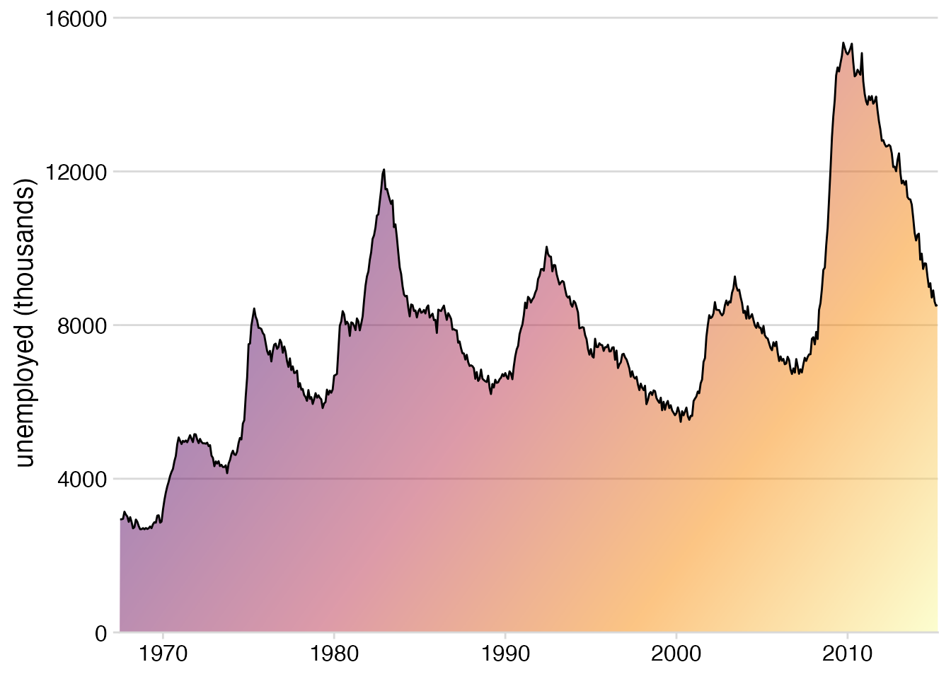
# define a radial gradient object
radial_inferno <- radialGradient(
  colours = rev(c("#000004FF", "#56106EFF", "#BB3754FF", "#F98C0AFF", "#FCFFA4FF")),
  cx1 = 0.55, cx2 = 0.55,
  cy1 = 0.25, cy2 = 0.25,
  group = FALSE
)

ggplot(economics, aes(date, unemploy)) +
  geom_area(fill = radial_inferno, alpha = 0.5) +
  geom_line() +
  scale_x_date(
    name = NULL,
    expand = expansion(mult = c(0, 0))
  ) +
  scale_y_continuous(
    name = "unemployed (thousands)",
    expand = expansion(mult = c(0, 0.05))
  ) +
  theme_minimal_hgrid()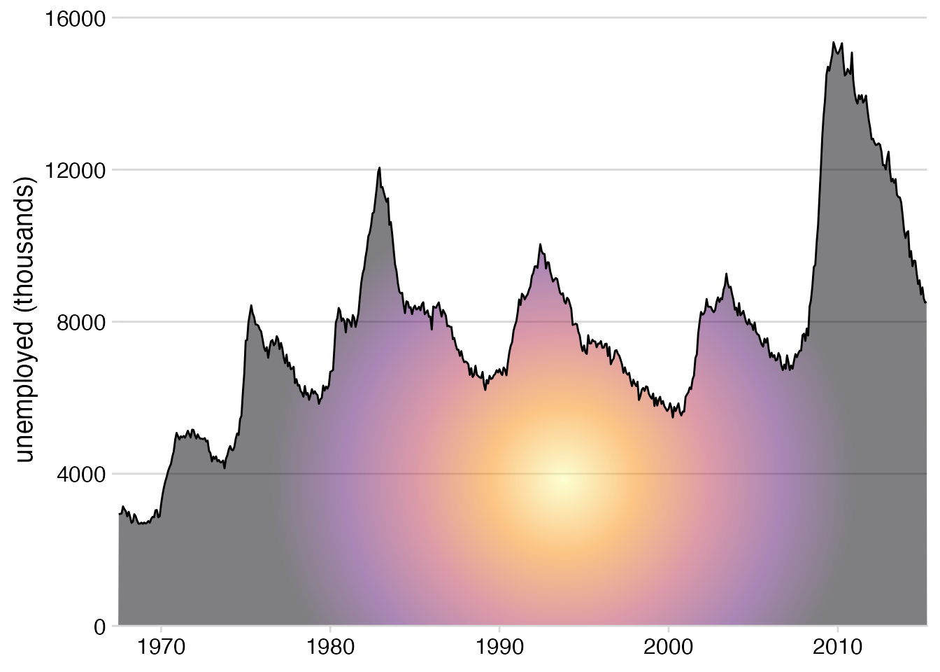
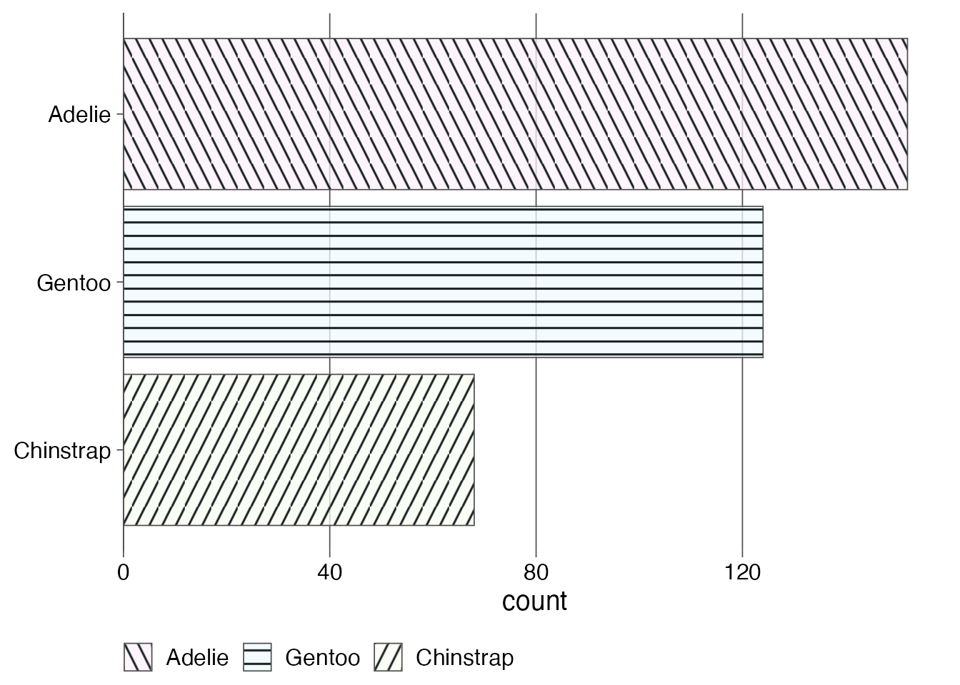
Exercise 1.2: Make your own patterns for the bar plot with pattern fill.
crosshatch1 <- pattern(
  grobTree(
    rectGrob(gp = gpar(fill = "#FAFEF0C0", col = NA)),
    segmentsGrob(
      x0 = c(0, 0.5), y0 = c(0, 0),
      x1 = c(0.5, 1), y1 = c(1, 1),
      gp = gpar(col = "#182124", lwd = 1.5)
    ),
    vp = viewport(width = unit(5, "mm"), height = unit(5, "mm"))
  ),
  width = unit(5, "mm"), height = unit(5, "mm"),
  extend = "repeat"
)

crosshatch2 <- pattern(
  grobTree(
    rectGrob(gp = gpar(fill = "#F0FAFEC0", col = NA)),
    segmentsGrob(
      x0 = c(0, 0), y0 = c(0.25, 0.75),
      x1 = c(1, 1), y1 = c(0.25, 0.75),
      gp = gpar(col = "#182124", lwd = 1.5)
    ),
    vp = viewport(width = unit(5, "mm"), height = unit(5, "mm"))
  ),
  width = unit(5, "mm"), height = unit(5, "mm"),
  extend = "repeat"
)

crosshatch3 <- pattern(
  grobTree(
    rectGrob(gp = gpar(fill = "#FEF0FAC0", col = NA)),
    segmentsGrob(
      x0 = c(0, 0.5), y0 = c(1, 1),
      x1 = c(0.5, 1), y1 = c(0, 0),
      gp = gpar(col = "#182124", lwd = 1.5)
    ),
    vp = viewport(width = unit(5, "mm"), height = unit(5, "mm"))
  ),
  width = unit(5, "mm"), height = unit(5, "mm"),
  extend = "repeat"
)

patterns <- list(
  crosshatch1, crosshatch2, crosshatch3
)

penguins |>
  count(species) |>
  mutate(species = fct_reorder(species, n)) |>
  ggplot(aes(n, species, fill = species)) +
  geom_col(color = "gray30", linewidth = 0.3) +
  scale_fill_manual(
    name = NULL,
    # here we're using patterns instead of colors
    values = patterns,
    guide = guide_legend(
      position = "bottom",
      reverse = TRUE
    )
  ) +
  scale_x_continuous(
    name = "count",
    expand = expansion(mult = c(0, 0.05))
  ) +
  scale_y_discrete(
    name = NULL
  ) +
  theme_minimal_vgrid(
    color = "gray30",
    line_size = 0.3
  )
Solutions, Section 2
Data preparation:
# data taken from: https://github.com/john-guerra/US_Elections_Results/tree/master
votes_2016 <- read_csv("https://wilkelab.org/dataviz_shortcourse/datasets/2016_US_County_Level_Presidential_Results.csv") |>
  mutate(
    fips = str_pad(combined_fips, 5, pad = "0"),
    state = state_abbr
  )

votes_long <- votes_2016 |>
  mutate(
    other = total_votes - votes_dem - votes_gop
  ) |>
  select(
    state, fips, democratic = votes_dem, republican = votes_gop, other
  ) |>
  pivot_longer(c(-state, -fips), names_to = "party", values_to = "votes")

# load geometry data
counties <- readRDS(url("https://wilkelab.org/dataviz_shortcourse/datasets/US_counties.rds")) |>
  mutate(
    fips = as.character(GEOID),
    state = state_code
  )
Exercise 2.1: Use side-by-side bar plots instead of pie charts.
Solution: First we generate the patterns.
make_bar_plot <- function(data) {
  data |>
    mutate(
      party = fct_relevel(party, 'republican', 'democratic', 'other')
    ) |>
    ggplot() +
    aes("", votes, fill = party) +
    geom_col(color = "black", linewidth = 0.2, position = "dodge") +
    scale_fill_manual(
      values = c(democratic = '#4B77D0', republican = '#DB4940', other = "gray70"),
      guide = "none"
    ) +
    theme_void()
}

make_bar_pattern <- function(data) {
  p <- make_bar_plot(data)
  pattern(
    ggplotGrob(p),
    extend = "none",
    group = FALSE
  )
}

vote_bars <- votes_long |>
  filter(state == "WY") |>
  select(-state) |>
  nest(data = -fips) |>
  mutate(
    bar_pattern = map(data, make_bar_pattern),
    vote_total = map_dbl(data, ~sum(.x$votes))
  ) |>
  select(-data)
Then we make the plot.
counties |>
  filter(state == "WY") |>
  mutate( # calculate reference point for each county
    points = st_point_on_surface(st_zm(geometry)),
    county_x = st_coordinates(points)[, "X"],
    county_y = st_coordinates(points)[, "Y"]
  ) |>
  left_join(vote_bars, by = "fips") |>
  mutate( # calculate plot scale
    scale = 1.2 * vote_total,
  ) |>
  ggplot() +
  geom_sf(color = "gray40", fill = "gray95", linewidth = 0.2) +
  geom_rect(
    aes(
      geometry = geometry,
      xmin = county_x - 25000,
      xmax = county_x + 25000,
      ymin = county_y - .5 * scale,
      ymax = county_y + 1.5 * scale,
      fill = bar_pattern
    ),
    stat = "sf_coordinates"
  ) +
  theme_void()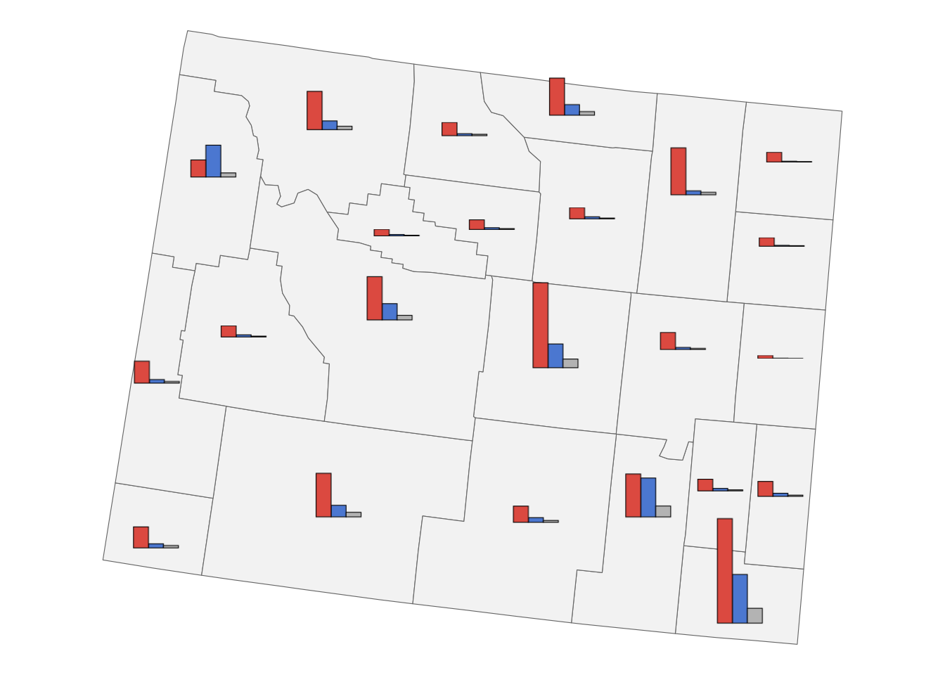
Solutions, Section 3
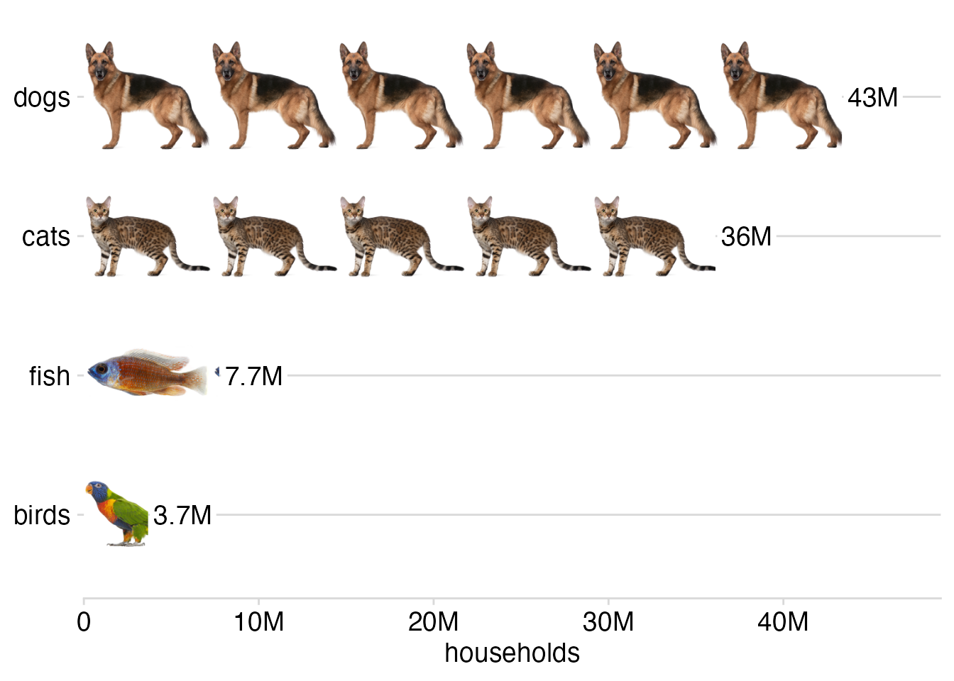
Exercise 3.1: Create a version of the pet ownership isotype plot where bars run vertical instead of horizontal.
make_img_pattern <- function(img) {
  pattern(
    rasterGrob(
      y = 0, vjust = 0, # needed to bottom-align the images
      magick::image_read(img),
      width = unit(20, "mm"),
      height = unit(20, "mm"),
      interpolate = FALSE,
    ),
    y = 0, vjust = 0, # needed to bottom-align the images
    width = unit(100, "mm"),
    height = unit(20, "mm"),
    extend = "repeat",
    group = FALSE
  )
}

patterns <- map(
  c(
    "https://wilkelab.org/dataviz_shortcourse/images/dog.png",
    "https://wilkelab.org/dataviz_shortcourse/images/cat.png",
    "https://wilkelab.org/dataviz_shortcourse/images/fish.png",
    "https://wilkelab.org/dataviz_shortcourse/images/bird.png"
  ),
  make_img_pattern
)

# data source: 2012 U.S. Pet Ownership & Demographics Sourcebook,
# American Veterinary Medical Association
pet_ownership <- read.table(text = "pet  households
dogs 43346000
cats 36117000
fish    7738000
birds 3671000
", header = TRUE)

pet_ownership |>
  mutate(
    pet = fct_reorder(pet, -households)
  ) |>
  ggplot() +
  aes(x = pet, y = households, fill = pet) +
  geom_col() +
  geom_label(
    aes(label = paste0(signif(households*1e-6, 2), "M")),
    hjust = 0.5,
    vjust = 0,
    nudge_y = .1e6,
    size = 14,
    size.unit = "pt",
    label.size = 0, # no label outline
    label.padding = unit(2, "pt"),
    fill = "#FFFFFF"
  ) +
  scale_y_continuous(
    limits = 1e6*c(0, 49),
    breaks = 1e7*(0:4),
    labels = c("0", paste0(10*(1:4), "M")),
    name = "households",
    expand = c(0, 0)
  ) +
  scale_x_discrete(
    name = NULL
  ) +
  scale_fill_manual(
    values = patterns,
    guide = "none"
  ) +
  theme_minimal_hgrid(rel_small = 1)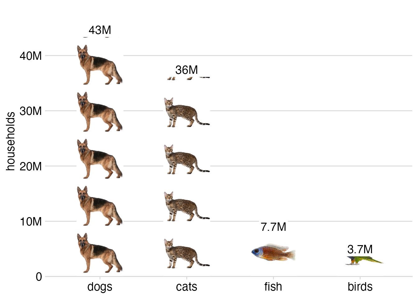
- Recreate the pet ownership isotype plot with ggpattern.
library(ggpattern)

pet_images <- c(
  "https://wilkelab.org/dataviz_shortcourse/images/bird.png",
  "https://wilkelab.org/dataviz_shortcourse/images/fish.png",
  "https://wilkelab.org/dataviz_shortcourse/images/cat.png",
  "https://wilkelab.org/dataviz_shortcourse/images/dog.png"
)

pet_ownership |>
  mutate(
    pet = fct_reorder(pet, households)
  ) |>
  ggplot() +
  aes(y = pet, x = households) +
  geom_col_pattern(
    aes(
      pattern_filename = pet
    ),
    pattern         = 'image',
    pattern_type    = 'tile',
    fill            = 'white',
    colour          = NA,
    pattern_filter  = 'box',
    pattern_scale   = -2
  ) +
  geom_label(
    aes(label = paste0(signif(households*1e-6, 2), "M")),
    vjust = 0.5,
    hjust = 0,
    nudge_x = .1e6,
    size = 14,
    size.unit = "pt",
    label.size = 0, # no label outline
    label.padding = unit(2, "pt"),
    fill = "#FFFFFF"
  ) +
  scale_x_continuous(
    limits = 1e6*c(0, 49),
    breaks = 1e7*(0:4),
    labels = c("0", paste0(10*(1:4), "M")),
    name = "households",
    expand = c(0, 0)
  ) +
  scale_y_discrete(
    name = NULL
  ) +
  scale_pattern_filename_discrete(
    choices = pet_images,
    guide = "none"
  ) +
  theme_minimal_hgrid(rel_small = 1)