Sample outcomes from a fitted model

Sample outcomes from a fitted model (via sample_outcomes()) or calculate a confidence band for the fitted model (via confidence_band()). Currently, sampling of fitted models is only implemented for generalized additive models fitted with mgcv::gam().

sample_outcomes(model, newdata, times = 20, key = ".draw", ...)

# S3 method for gam
sample_outcomes(model, newdata, times = 20,
  key = ".draw", unconditional = FALSE, ...)

confidence_band(model, newdata, level = 0.95, ...)

# S3 method for gam
confidence_band(model, newdata, level = 0.95,
  unconditional = FALSE, ...)

Arguments

model	The fitted model to use for generating outcomes or calculating a confidence band.
newdata	A data frame containing the values of the model covariates at which outcomes or confidence values should be calculated, as in `predict.gam()`.
times	Number of times outcomes should be drawn.
key	Character vector holding the name of the column indicating separate outcome draws. Default is `.draw`.
...	Other arguments.
unconditional	Bool indicating whether the smoothing parameter uncertainty corrected covariance matrix is used (`TRUE`) or not (`FALSE`, the default), as in `predict.gam()`. A choice of `unconditional = TRUE` will generally require the gam model to be fit by REML (`method = "REML"` in the `gam()` call).
level	Confidence level. Default is 95%.

Examples

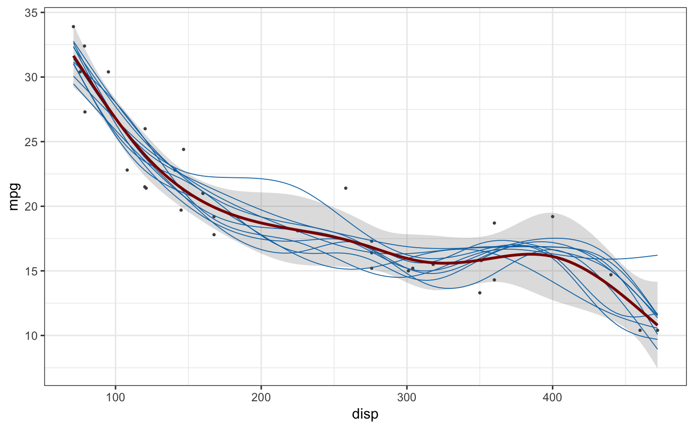
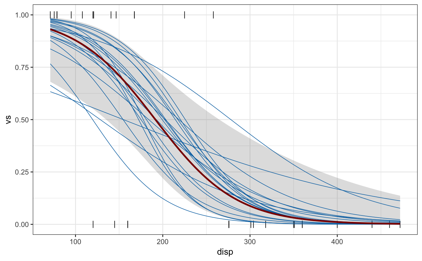
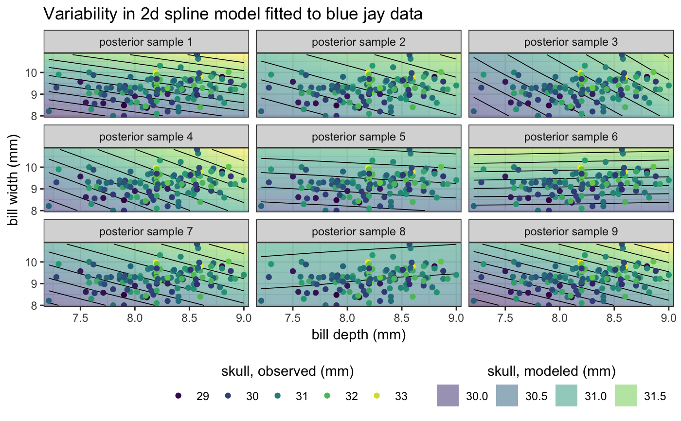
library(mgcv)
#> Loading required package: nlme
#> 
#> Attaching package: ‘nlme’
#> The following object is masked from ‘package:dplyr’:
#> 
#>     collapse
#> This is mgcv 1.8-24. For overview type 'help("mgcv-package")'.
library(ggplot2)

# gam spline fit
fit <- gam(mpg ~ s(disp), data = mtcars, method = "REML")

newdata <- data.frame(
  disp = seq(
    min(mtcars$disp), max(mtcars$disp),
    length.out = 100
  )
)

sample_df <- sample_outcomes(fit, newdata, 10, unconditional = TRUE)
conf <- confidence_band(fit, newdata, unconditional = TRUE)
ggplot(mtcars, aes(disp, mpg)) +
  geom_ribbon(data = conf, aes(ymin = lo, ymax = hi), fill="#80808040", color = NA) +
  geom_point(color = "grey30", size = 0.5) +
  geom_line(data = sample_df, aes(group = .draw), color = "#0072B2", size = 0.3) +
  geom_line(data = conf, size = 1, color = "darkred") +
  theme_bw()

# logistic regression fit
fit <- gam(vs ~ disp, data = mtcars, family = "binomial")

sample_df <- sample_outcomes(fit, newdata, 20)
conf <- confidence_band(fit, newdata)
ggplot(mtcars, aes(disp, vs)) +
  geom_ribbon(data = conf, aes(ymin = lo, ymax = hi), fill="#80808040", color = NA) +
  geom_point(color = "black", size = 3, shape = "|") +
  geom_line(data = sample_df, aes(group = .draw), color = "#0072B2", size = 0.3) +
  geom_line(data = conf, size = 1, color = "darkred") +
  theme_bw()

# example in 2D
data(BlueJays, package = "Stat2Data")

fit <- gam(Skull ~ s(BillDepth, BillWidth), data = BlueJays, method = "REML")

newdata <- expand.grid(
  BillWidth = seq(min(BlueJays$BillWidth), max(BlueJays$BillWidth), length.out = 20),
  BillDepth = seq(min(BlueJays$BillDepth), max(BlueJays$BillDepth), length.out = 20)
)

sample_df <- sample_outcomes(fit, newdata, 9, unconditional = TRUE)
ggplot(BlueJays, aes(BillDepth, BillWidth)) +
  geom_tile(data = sample_df, aes(fill = Skull), alpha = 0.5, color = NA) +
  geom_contour(data = sample_df, aes(z = Skull), color = "black", size = 0.3, binwidth = 0.2) +
  geom_point(aes(color = Skull), size = 1.5) +
  scale_fill_viridis_c(
    name = "skull, modeled (mm)",
    option = "D",
    guide = guide_legend(
      title.position = "top",
      order = 2,
      override.aes = list(alpha = 0.5)
    )
  ) +
  scale_color_viridis_c(
    name = "skull, observed (mm)",
    option = "D",
    guide = guide_legend(title.position = "top", order = 1)
  ) +
  coord_cartesian(expand = FALSE) +
  xlab("bill depth (mm)") +
  ylab("bill width (mm)") +
  ggtitle("Variability in 2d spline model fitted to blue jay data") +
  facet_wrap(~.draw, labeller = as_labeller(function(x) paste0("posterior sample ", x))) +
  theme_bw() +
  theme(
    legend.direction = "horizontal",
    legend.position = "bottom",
    legend.justification = "right",
    legend.title.align = 0.5
  )

Arguments

Examples

Contents