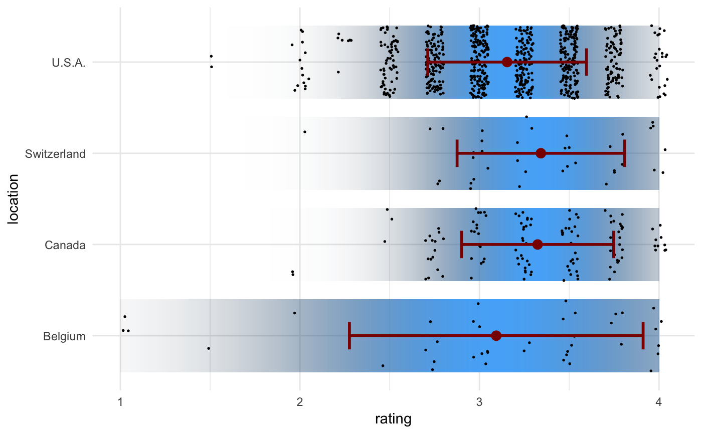
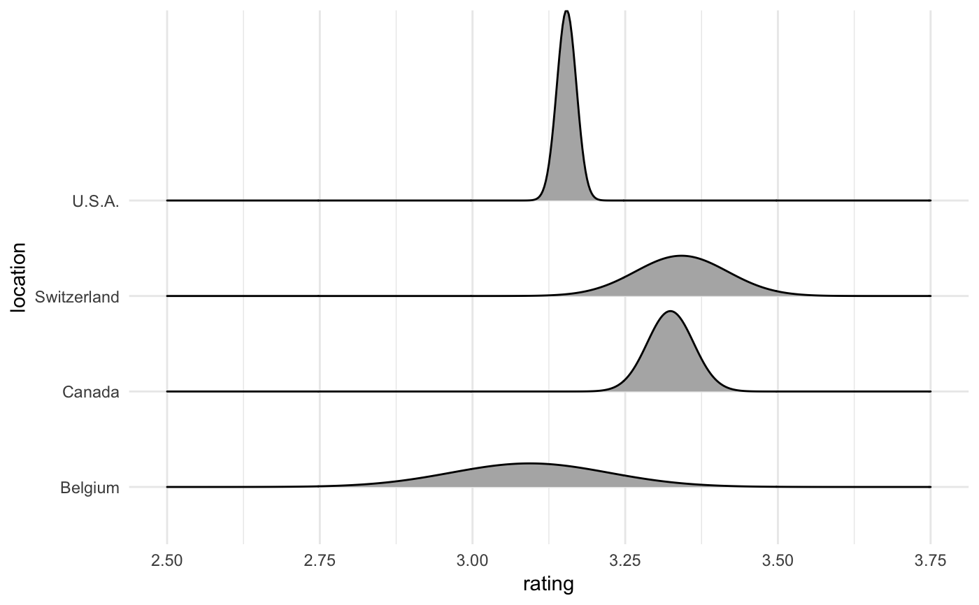
Confidence density distributions generated from estimate and margin of error

This stat generates normal densities from provided estimates plus margins of error (at a specified confidence level). It can be used to estimate the confidence density that underlies a given parameter estimate with given margin of error.

stat_confidence_density(mapping = NULL, data = NULL, geom = "tile",
  position = "identity", ..., confidence = 0.95, xlim = NULL,
  n = 501, na.rm = FALSE, show.legend = FALSE, inherit.aes = TRUE)

Arguments

mapping	Set of aesthetic mappings created by aes() or aes_(). If specified and inherit.aes = TRUE (the default), it is combined with the default mapping at the top level of the plot. You must supply mapping if there is no plot mapping.
data	The data to be displayed in this layer. There are three options: If NULL, the default, the data is inherited from the plot data as specified in the call to ggplot(). A data.frame, or other object, will override the plot data. All objects will be fortified to produce a data frame. See fortify() for which variables will be created. A function will be called with a single argument, the plot data. The return value must be a data.frame, and will be used as the layer data.
geom	The geometric object to use display the data
position	Position adjustment, either as a string, or the result of a call to a position adjustment function.
...	Other arguments passed on to layer(). These are often aesthetics, used to set an aesthetic to a fixed value, like colour = "red" or size = 3. They may also be parameters to the paired geom/stat.
confidence	The confidence level used to calculate the moe statistic. This defaults to 0.95 (moe corresponds to 95% confidence interval).
xlim	Numeric vector of two numbers setting the range of x values to be covered by the confidence density. If not supplied, is taken from the x scale.
n	Number of equally spaced points at which the density is calculated.
na.rm	If FALSE, the default, missing values are removed with a warning. If TRUE, missing values are silently removed.
show.legend	logical. Should this layer be included in the legends? NA, the default, includes if any aesthetics are mapped. FALSE never includes, and TRUE always includes. It can also be a named logical vector to finely select the aesthetics to display.
inherit.aes	If FALSE, overrides the default aesthetics, rather than combining with them. This is most useful for helper functions that define both data and aesthetics and shouldn't inherit behaviour from the default plot specification, e.g. borders().

Source

Adrian W. Bowman. Graphs for Uncertainty. J. R. Statist. Soc. A 182:1-16, 2018. http://www.rss.org.uk/Images/PDF/events/2018/Bowman-5-Sept-2018.pdf

Details

The following aesthetics are understood by this stat (required aesthetics are in bold):

• x: The estimate whose uncertainty is to be displayed

• moe: Margin of error

• confidence: Confidence level used to calculate the moe statistic. This defaults to 0.95 (moe corresponds to 95% confidence interval).

Examples

library(ggplot2)
library(dplyr)

cacao_small <- cacao %>%
  filter(location %in% c("Switzerland", "Canada", "U.S.A.", "Belgium"))

cacao_summary <- cacao_small %>%
  group_by(location) %>%
  summarize(
    sd = sd(rating),
    moe = sd*1.96,
    rating = mean(rating)
  )

ggplot(cacao_summary, aes(x = rating, y = location)) +
  stat_confidence_density(aes(moe = moe, fill = stat(ndensity)), height = 0.8) +
  geom_point(data = cacao_small, position = position_jitter(width = 0.05), size = 0.3) +
  geom_errorbarh(
    aes(xmin = rating - sd, xmax = rating + sd),
    height = 0.3, color = "darkred", size = 1
  ) +
  geom_point(size = 3, color = "darkred") +
  theme_minimal()


library(ggridges)
#> 
#> Attaching package: ‘ggridges’
#> The following object is masked from ‘package:ggplot2’:
#> 
#>     scale_discrete_manual

cacao_se <- cacao_small %>%
  group_by(location) %>%
  summarize(
    se = sd(rating)/sqrt(n()),
    moe = se*1.96,
    rating = mean(rating)
  )

ggplot(cacao_se, aes(x = rating, y = location)) +
  stat_confidence_density(
    geom = "ridgeline",
    aes(moe = moe, height = stat(density)),
    alpha = NA, xlim = c(2.5, 3.75), scale = 0.08
  ) +
  theme_minimal()