The ggtext package defines two new geoms, geom_richtext() and geom_textbox(), which can be used to plot with markdown text. They draw simple text labels (without word wrap) and textboxes (with word wrap), respectively.
Simple text labels
Markdown-formatted text labels can be placed into a plot with geom_richtext(). This geom is mostly a drop-in replacement for geom_label() (or geom_text()), with added capabilities.
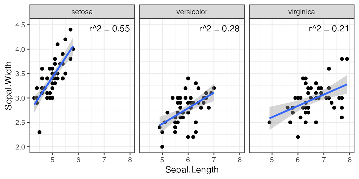
As a first example, we will annotate a plot of linear regressions with their r2 values. We will use the iris dataset for this demonstration. In our first iteration, we will not yet use any ggtext features, and instead plot the text with geom_text().
library(ggplot2)
library(dplyr)
library(glue)

iris_cor <- iris %>%
  group_by(Species) %>%
  summarize(r_square = cor(Sepal.Length, Sepal.Width)^2) %>%
  mutate(
    # location of each text label in data coordinates
    Sepal.Length = 8, Sepal.Width = 4.5,
    # text label containing r^2 value
    label = glue("r^2 = {round(r_square, 2)}")
  )

iris_cor
#> # A tibble: 3 x 5
#>   Species    r_square Sepal.Length Sepal.Width label
#>   <fct>         <dbl>        <dbl>       <dbl> <glue>
#> 1 setosa        0.551            8         4.5 r^2 = 0.55
#> 2 versicolor    0.277            8         4.5 r^2 = 0.28
#> 3 virginica     0.209            8         4.5 r^2 = 0.21

iris_facets <- ggplot(iris, aes(Sepal.Length, Sepal.Width)) +
  geom_point() +
  geom_smooth(method = "lm", formula = y ~ x) +
  facet_wrap(~Species) +
  theme_bw()

iris_facets +
  geom_text(
    data = iris_cor,
    aes(label = label),
    hjust = 1, vjust = 1
  )
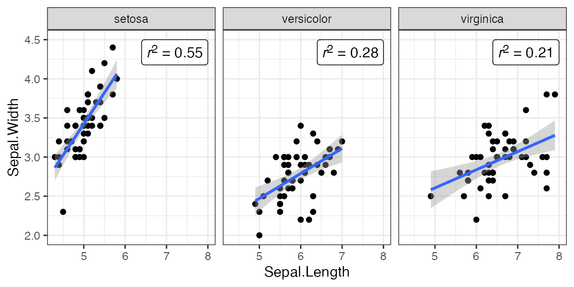
This code works, but the result is not fully satisfying. First, because r is a mathematical variable, it should be typeset in italics. Second, it would be nicer to have a superscript 2 instead of ^2. We can achieve both results by creating a markdown label and plotting it with geom_richtext().
library(ggtext)

iris_cor_md <- iris_cor %>%
  mutate(
    # markdown version of text label
    label = glue("*r*<sup>2</sup> = {round(r_square, 2)}")
  )

iris_cor_md
#> # A tibble: 3 x 5
#>   Species    r_square Sepal.Length Sepal.Width label
#>   <fct>         <dbl>        <dbl>       <dbl> <glue>
#> 1 setosa        0.551            8         4.5 *r*<sup>2</sup> = 0.55
#> 2 versicolor    0.277            8         4.5 *r*<sup>2</sup> = 0.28
#> 3 virginica     0.209            8         4.5 *r*<sup>2</sup> = 0.21

iris_facets +
  geom_richtext(
    data = iris_cor_md,
    aes(label = label),
    hjust = 1, vjust = 1
  )
By default, geom_richtext() puts a box around the text it draws. We can suppress the box by setting the fill and outline colors to transparent (fill = NA, label.colour = NA).
iris_facets +
  geom_richtext(
    data = iris_cor_md,
    aes(label = label),
    hjust = 1, vjust = 1,
    # remove label background and outline
    fill = NA, label.color = NA,
    # remove label padding, since we have removed the label outline
    label.padding = grid::unit(rep(0, 4), "pt")
  )

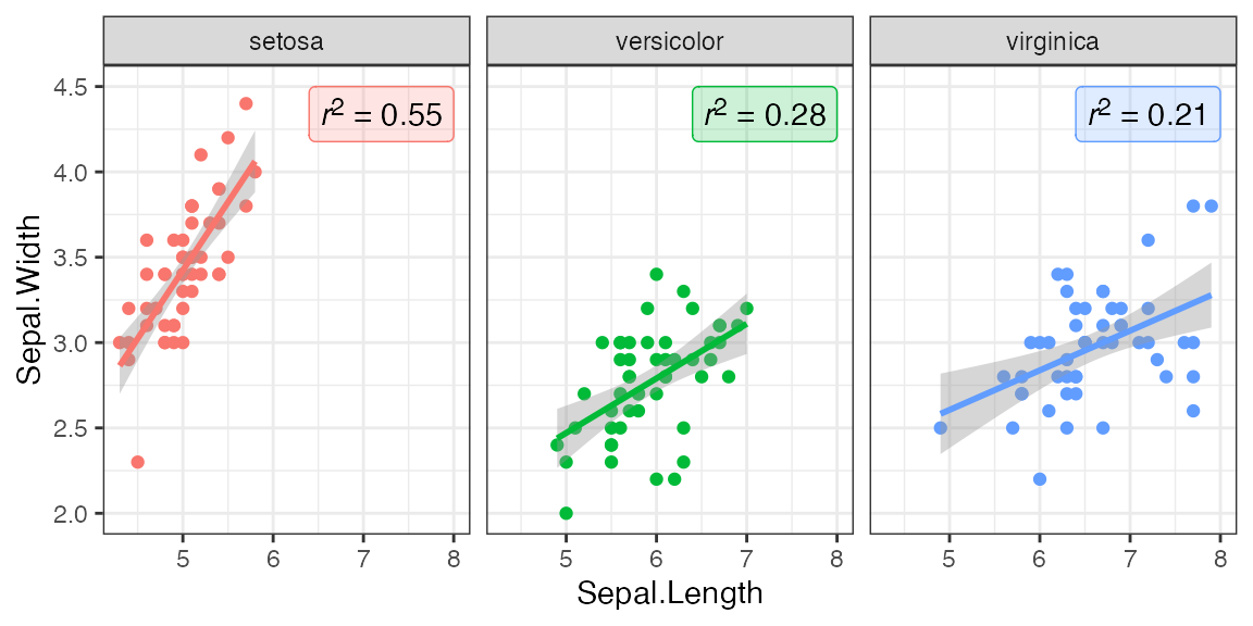
We can separately choose the colors of label outline, label fill, and label text, and we can assign them via aesthetic mapping as well as by direct specification, as is usual in ggplot2.
iris_facets +
  aes(colour = Species) +
  geom_richtext(
    data = iris_cor_md,
    aes(
      label = label,
      fill = after_scale(alpha(colour, .2))
    ),
    text.colour = "black",
    hjust = 1, vjust = 1
  ) +
  theme(legend.position = "none")
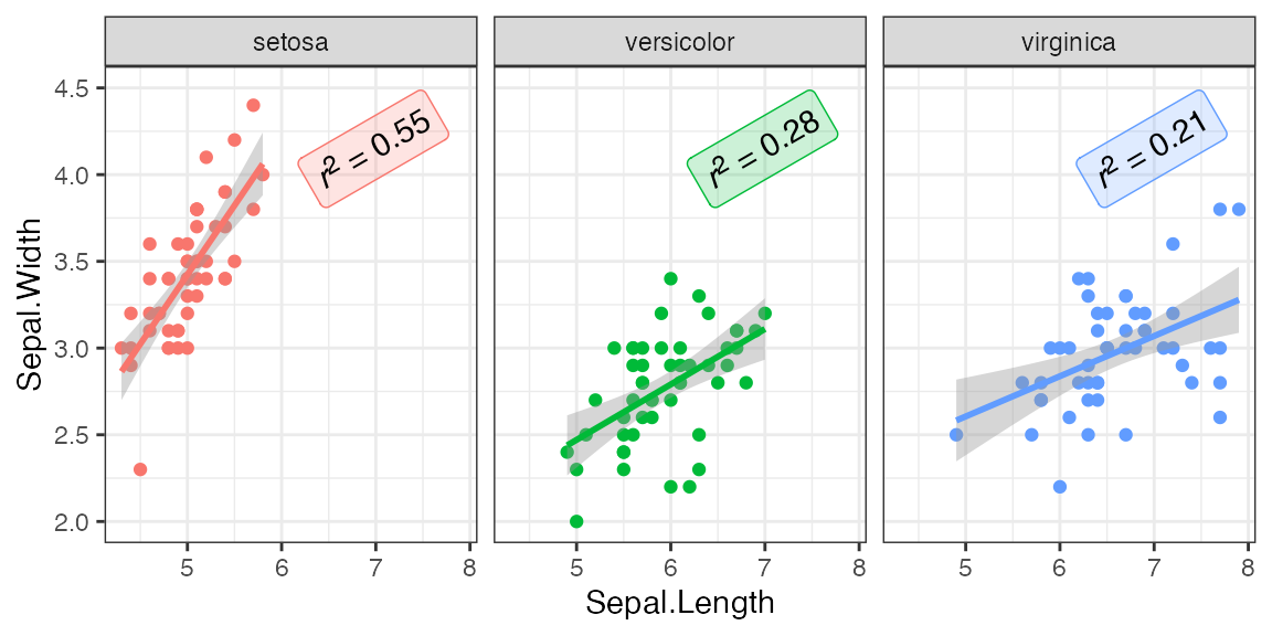
Rotated labels are also possible, though in most cases it is not recommended to use them.
iris_facets +
  aes(colour = Species) +
  geom_richtext(
    data = iris_cor_md,
    aes(
      x = 7.5,
      label = label,
      fill = after_scale(alpha(colour, .2))
    ),
    text.colour = "black",
    hjust = 1, vjust = 1,
    angle = 30
  ) +
  theme(legend.position = "none")
Text boxes
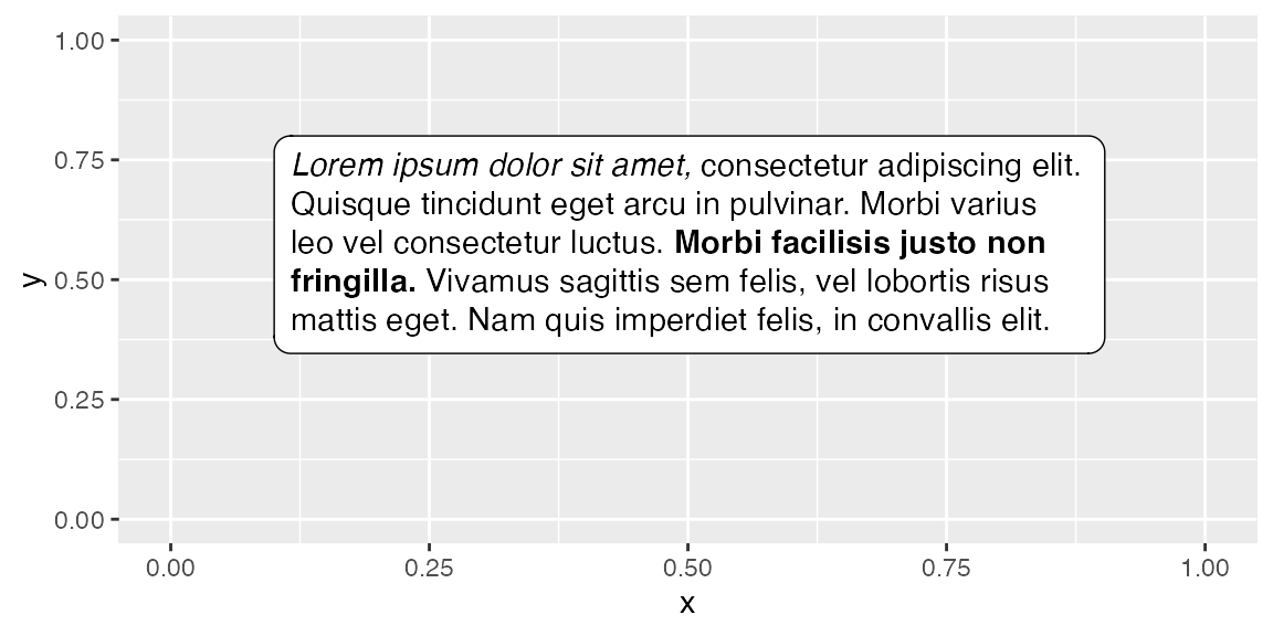
Markdown-formatted text boxes (with word wrap) can be placed into a plot with geom_textbox(). It is generally necessary to specify a width for the box. Widths are specified in grid units, and both absolute (e.g., "cm", "pt", or "in") and relative ("npc", Normalised Parent Coordinates) units are possible.
df <- data.frame(
  x = 0.1,
  y = 0.8,
  label = "*Lorem ipsum dolor sit amet,* consectetur adipiscing
elit. Quisque tincidunt eget arcu in pulvinar. Morbi varius leo
vel consectetur luctus. **Morbi facilisis justo non fringilla.**
Vivamus sagittis sem felis, vel lobortis risus mattis eget. Nam
quis imperdiet felis, in convallis elit."
)

p <- ggplot() +
  geom_textbox(
    data = df,
    aes(x, y, label = label),
    width = grid::unit(0.73, "npc"), # 73% of plot panel width
    hjust = 0, vjust = 1
  ) +
  xlim(0, 1) + ylim(0, 1)

p
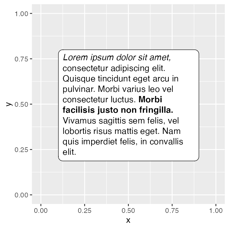
If we specify a relative width, then changing the size of the plot will change the size of the textbox. The text will reflow to accommodate this change.
p
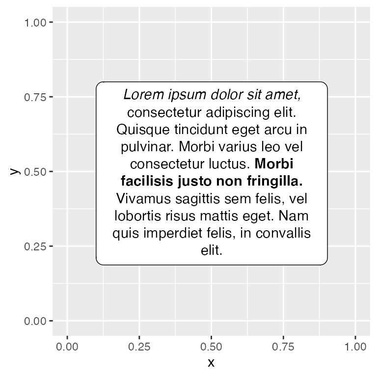
The parameters hjust and vjust align the box relative to the reference point specified by x and y, but they do not affect the alignment of text inside the box. To specify how text is aligned inside the box, use halign and valign. For example, halign = 0.5 generates centered text.
ggplot() +
  geom_textbox(
    data = df,
    aes(x, y, label = label),
    width = grid::unit(0.73, "npc"), # 73% of plot panel width
    hjust = 0, vjust = 1,
    halign = 0.5 # centered text
  ) +
  xlim(0, 1) + ylim(0, 1)
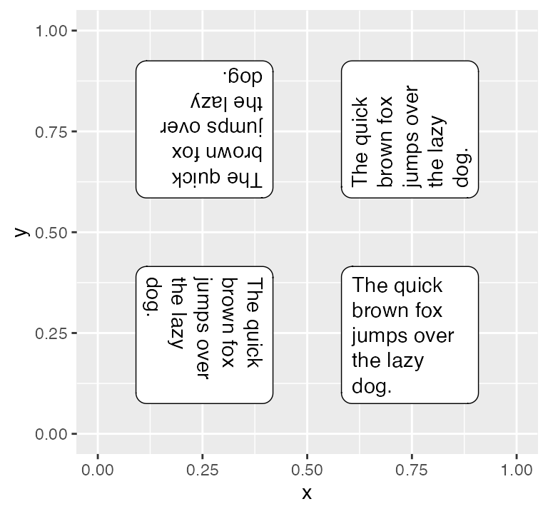
While text boxes cannot be rotated arbitrarily, they can be placed in four distinct orientations, corresponding to rotations by multiples of 90 degrees. Note that hjust and vjust are specified relative to this orientation.
df <- data.frame(
  x = 0.5,
  y = 0.5,
  label = "The quick brown fox jumps over the lazy dog.",
  orientation = c("upright", "left-rotated", "inverted", "right-rotated")
)

ggplot() +
  geom_textbox(
    data = df,
    aes(x, y, label = label, orientation = orientation),
    width = grid::unit(1.5, "in"),
    height = grid::unit(1.5, "in"),
    box.margin = grid::unit(rep(0.25, 4), "in"),
    hjust = 0, vjust = 1
  ) +
  xlim(0, 1) + ylim(0, 1) +
  scale_discrete_identity(aesthetics = "orientation")
The previous example uses the box.margin argument to create some space between the reference point given by x, y and the box itself. This margin is part of the size calculation for the box, so that a width of 1.5 inches with 0.25 inch margins yields an actual box of 1 inch in width.