Mixing different plotting frameworks

All cowplot functions that take plot objects as input (ggdraw(), draw_plot(), plot_grid()) can handle several different types of objects in addition to ggplot2 objects. Most importantly, they can handle plots produced with base R graphics. However, this functionality is only available if you have the package gridGraphics installed.

As the first example, we draw a base graphics plot with ggdraw() and style the background with the ggplot2 themeing mechanism.

library(ggplot2)
library(cowplot)

# define a function that emits the desired plot
p1 <- function() {
  par(
    mar = c(3, 3, 1, 1),
    mgp = c(2, 1, 0)
  )
  boxplot(mpg ~ cyl, xlab = "cyl", ylab = "mpg", data = mtcars)
}

ggdraw(p1) +
  theme(plot.background = element_rect(fill = "cornsilk"))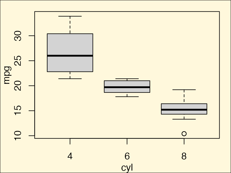

We can also add a logo to the plot.

logo_file <- system.file("extdata", "logo.png", package = "cowplot")

ggdraw() + 
  draw_image(
    logo_file,
    x = 1, width = 0.1,
    hjust = 1, halign = 1, valign = 0
  ) +
  draw_plot(p1)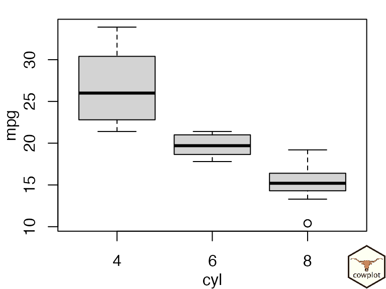

And we can draw base graphics and ggplot2 graphics side-by-side in a plot grid.

p2 <- ggplot(data = mtcars, aes(factor(cyl), mpg)) + geom_boxplot()
plot_grid(p1, p2)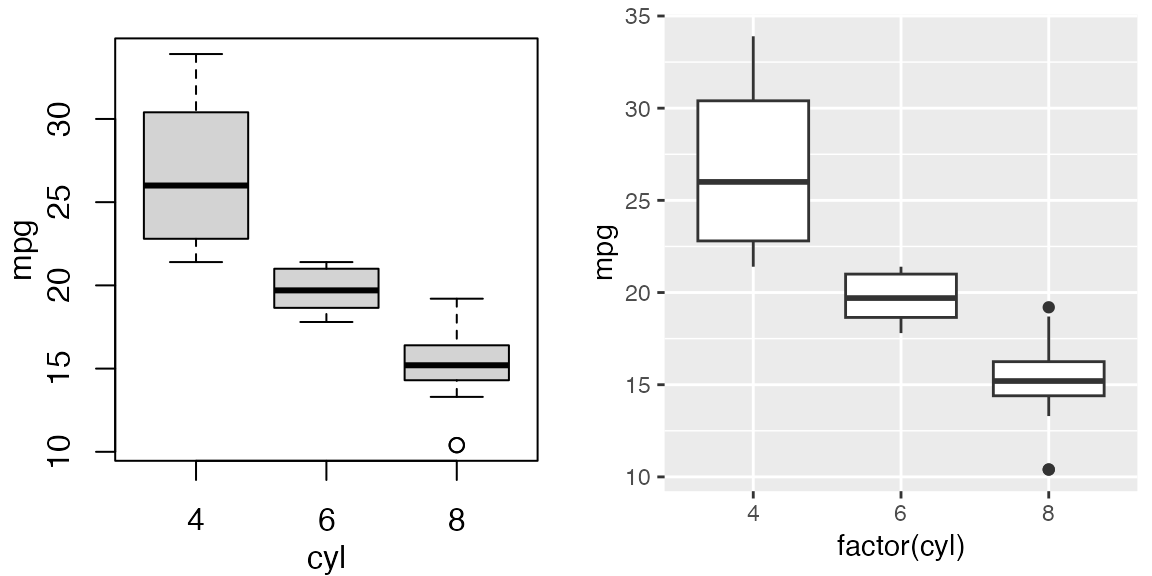

Base R plots can be stored in the form of functions that emit the desired plots (demonstrated above), as recorded plots, or using a convenient formula interface.

To create a recorded plot, we first draw the base plot, then we record it with recordPlot(), and then we can draw it with ggdraw().

# create base R plot
par(mar = c(3, 3, 1, 1), mgp = c(2, 1, 0))
boxplot(mpg ~ cyl, xlab = "cyl", ylab = "mpg", data = mtcars)

# record previous base R plot and then draw through ggdraw()
p1_recorded <- recordPlot()
ggdraw(p1_recorded)

We can store arbitrarily complex plotting code in formulas by enclosing it into curly braces.

# store base R plot as formula
p1_formula <- ~{
  par(
    mar = c(3, 3, 1, 1), 
    mgp = c(2, 1, 0)
  )
  boxplot(mpg ~ cyl, xlab = "cyl", ylab = "mpg", data = mtcars)
}
ggdraw(p1_formula)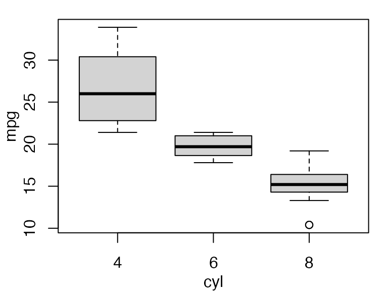

There is also support for lattice graphics and grid grobs.

# base R
p1 <- ~{
  par(
    mar = c(3, 3, 1, 1), 
    mgp = c(2, 1, 0)
  )
  boxplot(mpg ~ cyl, xlab = "cyl", ylab = "mpg", data = mtcars)
}

# ggplot2
p2 <- ggplot(data = mtcars, aes(factor(cyl), mpg)) + geom_boxplot()

# lattice
library(lattice)
p3 <- bwplot(~mpg | cyl, data = mtcars)

# elementary grid graphics objects
library(grid)
p4 <- circleGrob(r = 0.3, gp = gpar(fill = "skyblue"))

# combine all into one plot
plot_grid(p1, p2, p3, p4, rel_heights = c(.6, 1), labels = "auto")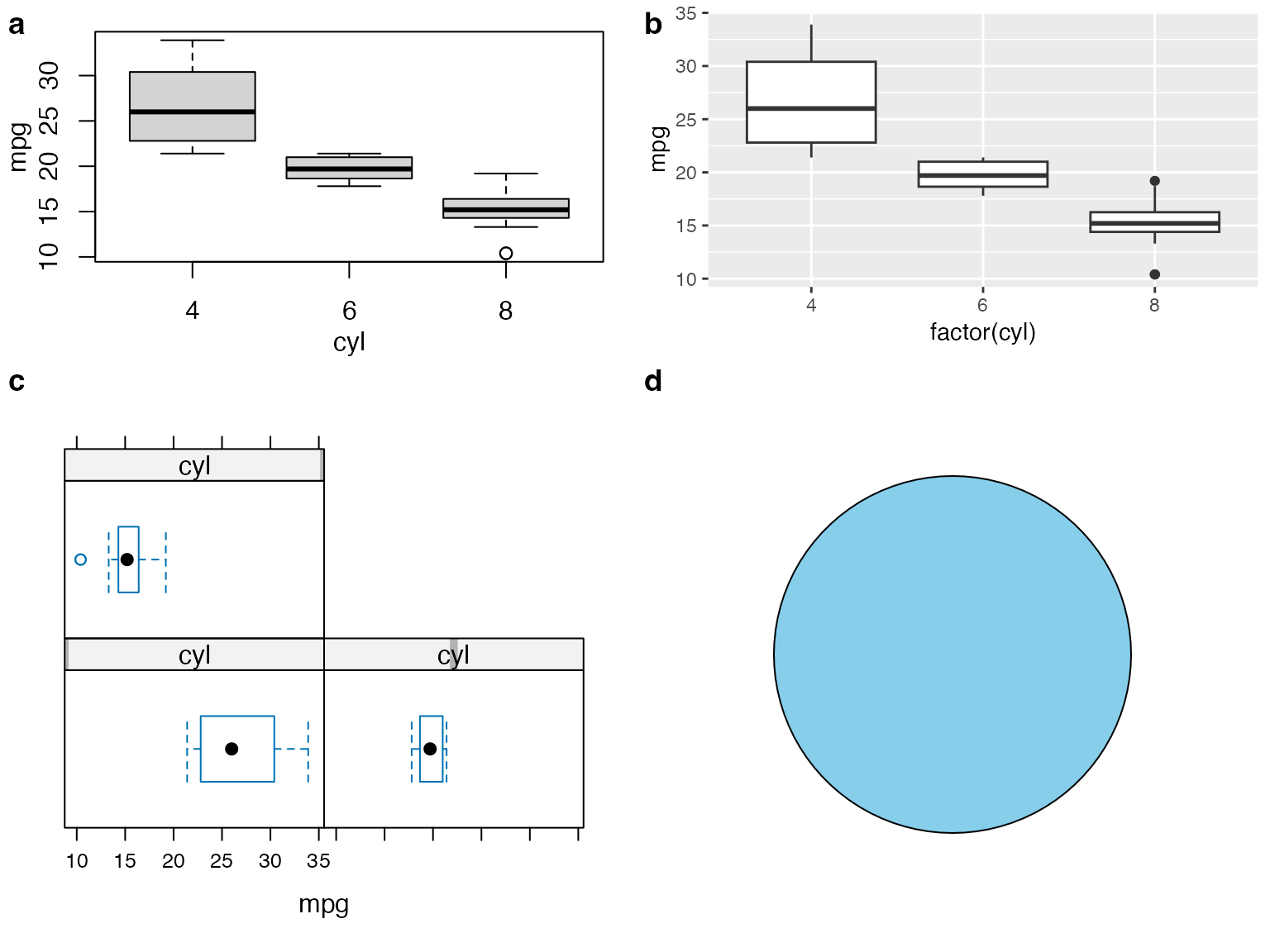

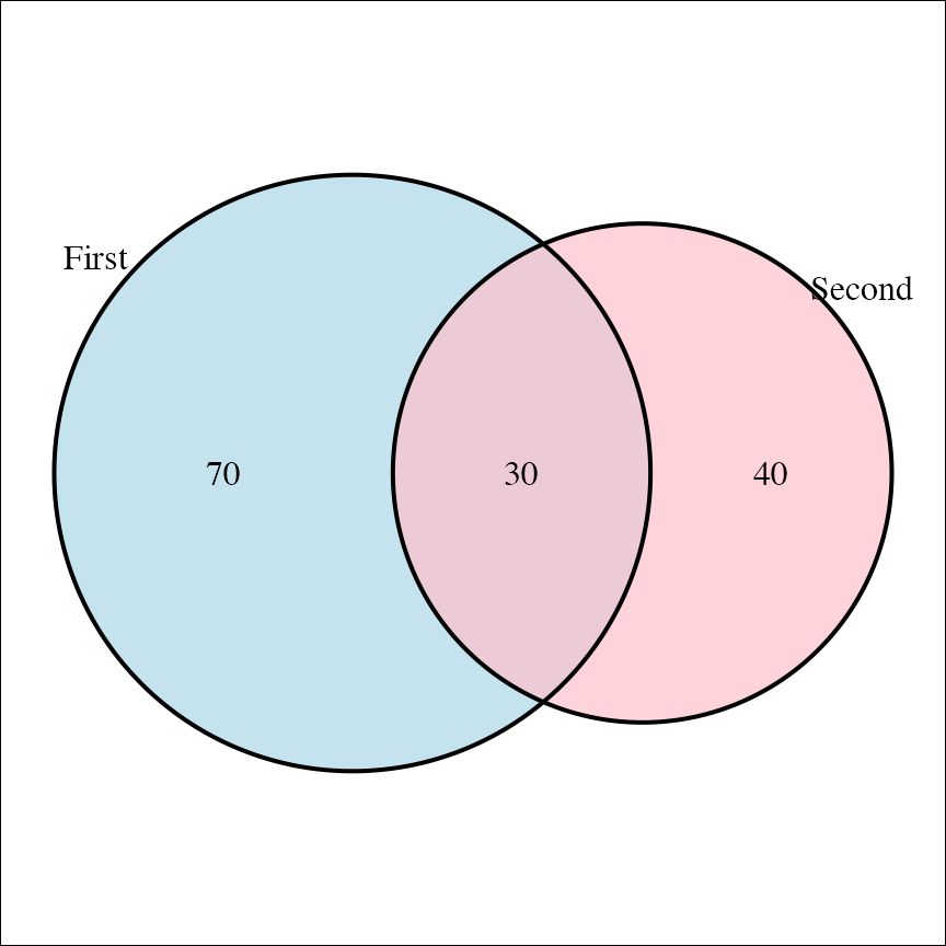
Other packages are supported as long as they return grid grobs.

library(VennDiagram)

p_venn <- draw.pairwise.venn(
  100, 70, 30,
  c("First", "Second"),
  fill = c("light blue", "pink"),
  alpha = c(0.7, 0.7),
  ind = FALSE
)

# plot venn diagram and add some margin and enclosing box
ggdraw(p_venn) +
  theme(
    plot.background = element_rect(fill = NA),
    plot.margin = margin(12, 12, 12, 12)
  )

Claus O. Wilke

2024-01-22