Stat for histogram ridgeline plots — stat

Works like stat_bin except that the output is a ridgeline describing the histogram rather than a set of counts.

Usage

stat_binline(
  mapping = NULL,
  data = NULL,
  geom = "density_ridges",
  position = "identity",
  ...,
  binwidth = NULL,
  bins = NULL,
  center = NULL,
  boundary = NULL,
  breaks = NULL,
  closed = c("right", "left"),
  pad = TRUE,
  draw_baseline = TRUE,
  na.rm = FALSE,
  show.legend = NA,
  inherit.aes = TRUE
)

Arguments

mapping

Set of aesthetic mappings created by aes(). If specified and inherit.aes = TRUE (the default), it is combined with the default mapping at the top level of the plot. You must supply mapping if there is no plot mapping.

data

The data to be displayed in this layer. There are three options:

If NULL, the default, the data is inherited from the plot data as specified in the call to ggplot().

A data.frame, or other object, will override the plot data. All objects will be fortified to produce a data frame. See fortify() for which variables will be created.

A function will be called with a single argument, the plot data. The return value must be a data.frame, and will be used as the layer data. A function can be created from a formula (e.g. ~ head(.x, 10)).

geom

The geom to use for drawing.

position

A position adjustment to use on the data for this layer. This can be used in various ways, including to prevent overplotting and improving the display. The position argument accepts the following:

The result of calling a position function, such as position_jitter(). This method allows for passing extra arguments to the position.
A string naming the position adjustment. To give the position as a string, strip the function name of the position_ prefix. For example, to use position_jitter(), give the position as "jitter".
For more information and other ways to specify the position, see the layer position documentation.

...

Other arguments passed on to layer()'s params argument. These arguments broadly fall into one of 4 categories below. Notably, further arguments to the position argument, or aesthetics that are required can not be passed through .... Unknown arguments that are not part of the 4 categories below are ignored.

Static aesthetics that are not mapped to a scale, but are at a fixed value and apply to the layer as a whole. For example, colour = "red" or linewidth = 3. The geom's documentation has an Aesthetics section that lists the available options. The 'required' aesthetics cannot be passed on to the params. Please note that while passing unmapped aesthetics as vectors is technically possible, the order and required length is not guaranteed to be parallel to the input data.
When constructing a layer using a stat_*() function, the ... argument can be used to pass on parameters to the geom part of the layer. An example of this is stat_density(geom = "area", outline.type = "both"). The geom's documentation lists which parameters it can accept.
Inversely, when constructing a layer using a geom_*() function, the ... argument can be used to pass on parameters to the stat part of the layer. An example of this is geom_area(stat = "density", adjust = 0.5). The stat's documentation lists which parameters it can accept.
The key_glyph argument of layer() may also be passed on through .... This can be one of the functions described as key glyphs, to change the display of the layer in the legend.

binwidth

The width of the bins. Can be specified as a numeric value or as a function that calculates width from unscaled x. Here, "unscaled x" refers to the original x values in the data, before application of any scale transformation. When specifying a function along with a grouping structure, the function will be called once per group. The default is to use the number of bins in bins, covering the range of the data. You should always override this value, exploring multiple widths to find the best to illustrate the stories in your data.

The bin width of a date variable is the number of days in each time; the bin width of a time variable is the number of seconds.

bins

Number of bins. Overridden by binwidth. Defaults to 30.

center, boundary

bin position specifiers. Only one, center or boundary, may be specified for a single plot. center specifies the center of one of the bins. boundary specifies the boundary between two bins. Note that if either is above or below the range of the data, things will be shifted by the appropriate integer multiple of binwidth. For example, to center on integers use binwidth = 1 and center = 0, even if 0 is outside the range of the data. Alternatively, this same alignment can be specified with binwidth = 1 and boundary = 0.5, even if 0.5 is outside the range of the data.

breaks

Alternatively, you can supply a numeric vector giving the bin boundaries. Overrides binwidth, bins, center, and boundary.

closed

One of "right" or "left" indicating whether right or left edges of bins are included in the bin.

pad

If TRUE, adds empty bins at either end of x. This ensures that the binline always goes back down to 0. Defaults to TRUE.

draw_baseline

If FALSE, removes lines along 0 counts. Defaults to TRUE.

na.rm

If FALSE, the default, missing values are removed with a warning. If TRUE, missing values are silently removed.

show.legend

logical. Should this layer be included in the legends? NA, the default, includes if any aesthetics are mapped. FALSE never includes, and TRUE always includes. It can also be a named logical vector to finely select the aesthetics to display.

inherit.aes

If FALSE, overrides the default aesthetics, rather than combining with them. This is most useful for helper functions that define both data and aesthetics and shouldn't inherit behaviour from the default plot specification, e.g. borders().

Examples

library(ggplot2)

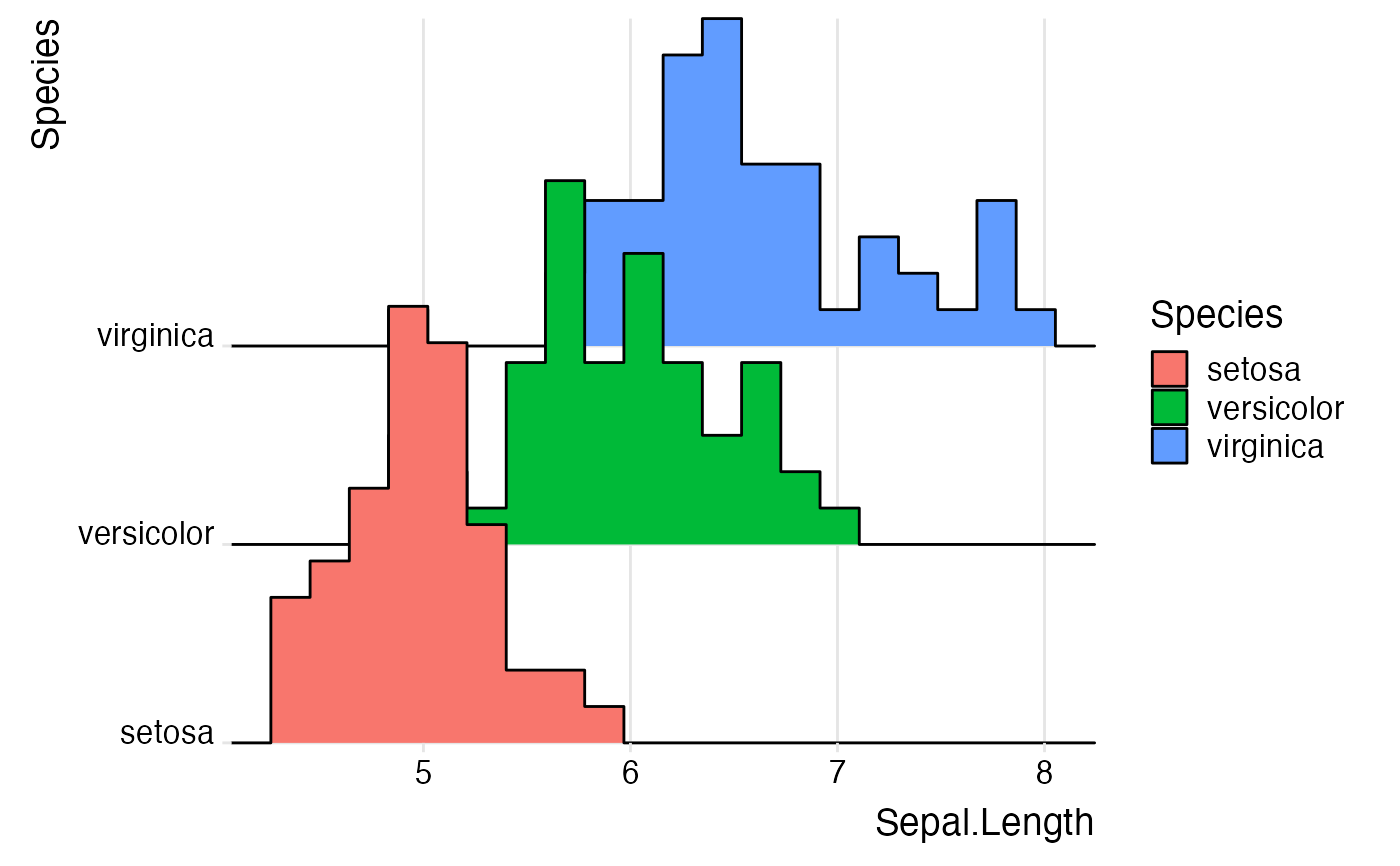
ggplot(iris, aes(x = Sepal.Length, y = Species, group = Species, fill = Species)) +
  geom_density_ridges(stat = "binline", bins = 20, scale = 2.2) +
  scale_y_discrete(expand = c(0, 0)) +
  scale_x_continuous(expand = c(0, 0)) +
  coord_cartesian(clip = "off") +
  theme_ridges()


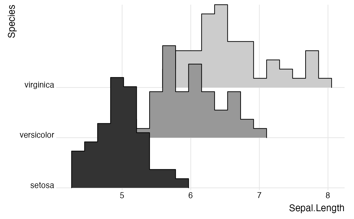
ggplot(iris, aes(x = Sepal.Length, y = Species, group = Species, fill = Species)) +
  stat_binline(bins = 20, scale = 2.2, draw_baseline = FALSE) +
  scale_y_discrete(expand = c(0, 0)) +
  scale_x_continuous(expand = c(0, 0)) +
  scale_fill_grey() +
  coord_cartesian(clip = "off") +
  theme_ridges() +
  theme(legend.position = 'none')


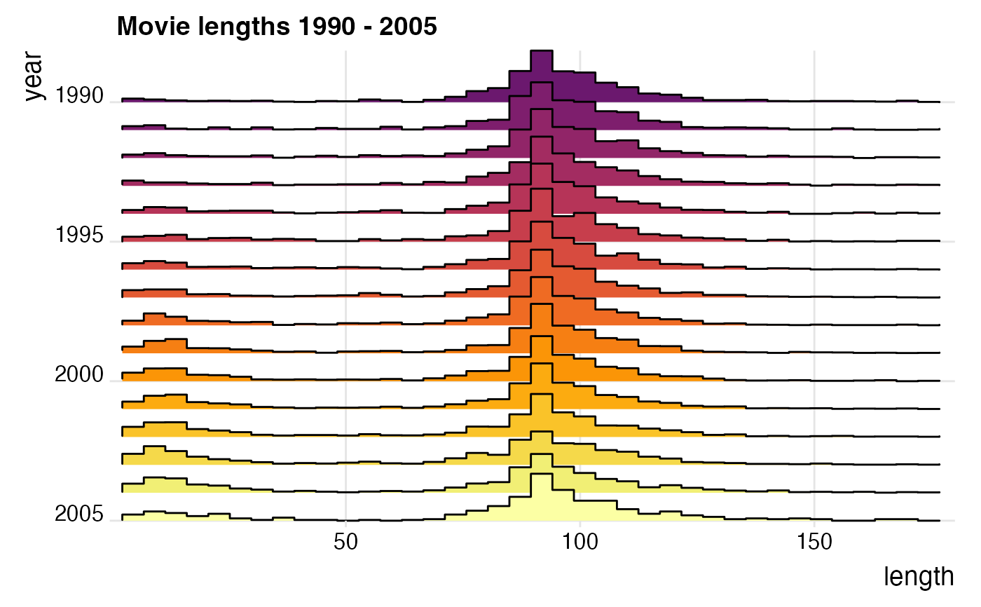
library(ggplot2movies)
ggplot(movies[movies$year>1989,], aes(x = length, y = year, fill = factor(year))) +
   stat_binline(scale = 1.9, bins = 40) +
   scale_x_continuous(limits = c(1, 180), expand = c(0, 0)) +
   scale_y_reverse(expand = c(0, 0)) +
   scale_fill_viridis_d(begin = 0.3, option = "B") +
   coord_cartesian(clip = "off") +
   labs(title = "Movie lengths 1990 - 2005") +
   theme_ridges() +
   theme(legend.position = "none")
#> Warning: Removed 118 rows containing non-finite outside the scale range
#> (`stat_binline()`).


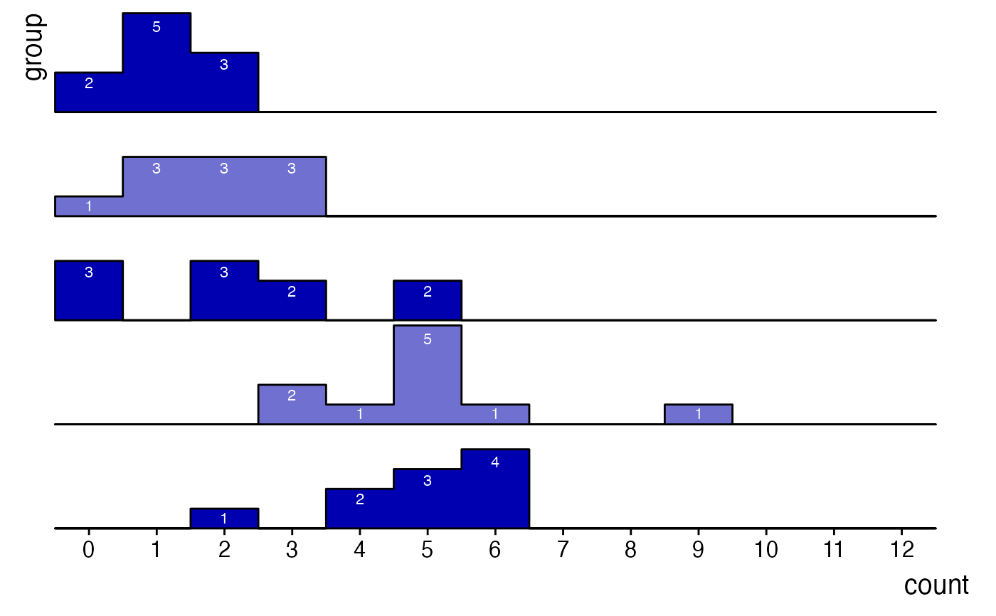
count_data <- data.frame(
  group = rep(letters[1:5], each = 10),
  mean = rep(1:5, each = 10)
)
count_data$group <- factor(count_data$group, levels = letters[5:1])
count_data$count <- rpois(nrow(count_data), count_data$mean)

ggplot(count_data, aes(x = count, y = group, group = group)) +
  geom_density_ridges2(
    stat = "binline",
    aes(fill = group),
    binwidth = 1,
    scale = 0.95
  ) +
  geom_text(
    stat = "bin",
    aes(y = group + 0.9*stat(count/max(count)),
    label = ifelse(stat(count) > 0, stat(count), "")),
    vjust = 1.2, size = 3, color = "white", binwidth = 1
  ) +
  scale_x_continuous(breaks = c(0:12), limits = c(-.5, 13), expand = c(0, 0)) +
  scale_y_discrete(expand = c(0, 0)) +
  scale_fill_cyclical(values = c("#0000B0", "#7070D0")) +
  guides(y = "none") +
  coord_cartesian(clip = "off") +
  theme_ridges(grid = FALSE)