This stat is the default stat used by geom_density_ridges. It is very similar to ggplot2::stat_density,
however there are a few differences. Most importantly, the density bandwidth is chosen across
the entire dataset.
Usage
stat_density_ridges(
  mapping = NULL,
  data = NULL,
  geom = "density_ridges",
  position = "identity",
  na.rm = FALSE,
  show.legend = NA,
  inherit.aes = TRUE,
  bandwidth = NULL,
  from = NULL,
  to = NULL,
  jittered_points = FALSE,
  quantile_lines = FALSE,
  calc_ecdf = FALSE,
  quantiles = 4,
  quantile_fun = quantile,
  n = 512,
  ...
)
Arguments
- mapping
Set of aesthetic mappings created by
ggplot2::aes(). If specified andinherit.aes = TRUE(the default), it is combined with the default mapping at the top level of the plot. You must supplymappingif there is no plot mapping.- data
The data to be displayed in this layer. There are three options:
If
NULL, the default, the data is inherited from the plot data as specified in the call toggplot().A
data.frame, or other object, will override the plot data.A
functionwill be called with a single argument, the plot data. The return value must be adata.frame., and will be used as the layer data.- geom
The geometric object to use to display the data.
- position
Position adjustment, either as a string, or the result of a call to a position adjustment function.
- na.rm
If
FALSE, the default, missing values are removed with a warning. IfTRUE, missing values are silently removed.- show.legend
logical. Should this layer be included in the legends?
NA, the default, includes if any aesthetics are mapped.FALSEnever includes, andTRUEalways includes.- inherit.aes
If
FALSE, overrides the default aesthetics, rather than combining with them.- bandwidth
Bandwidth used for density calculation. If not provided, is estimated from the data.
- from, to
The left and right-most points of the grid at which the density is to be estimated, as in
stats::density(). If not provided, these are estimated from the data range and the bandwidth.- jittered_points
If
TRUE, carries the original point data over to the processed data frame, so that individual points can be drawn by the various ridgeline geoms. The specific position of these points is controlled by various position objects, e.g.position_points_sina()orposition_raincloud().- quantile_lines
If
TRUE, enables the drawing of quantile lines. Overrides thecalc_ecdfsetting and sets it toTRUE.- calc_ecdf
If
TRUE,stat_density_ridgescalculates an empirical cumulative distribution function (ecdf) and returns a variableecdfand a variablequantile. Both can be mapped onto aesthetics viastat(ecdf)andstat(quantile), respectively.- quantiles
Sets the number of quantiles the data should be broken into. Used if either
calc_ecdf = TRUEorquantile_lines = TRUE. Ifquantilesis an integer then the data will be cut into that many equal quantiles. If it is a vector of probabilities then the data will cut by them.- quantile_fun
Function that calculates quantiles. The function needs to accept two parameters, a vector
xholding the raw data values and a vectorprobsproviding the probabilities that define the quantiles. Default isquantile.- n
The number of equally spaced points at which the density is to be estimated. Should be a power of 2. Default is 512.
- ...
other arguments passed on to
ggplot2::layer(). These are often aesthetics, used to set an aesthetic to a fixed value, likecolor = "red"orlinewidth = 3. They may also be parameters to the paired geom/stat.
Examples
library(ggplot2)
# Examples of coloring by ecdf or quantiles
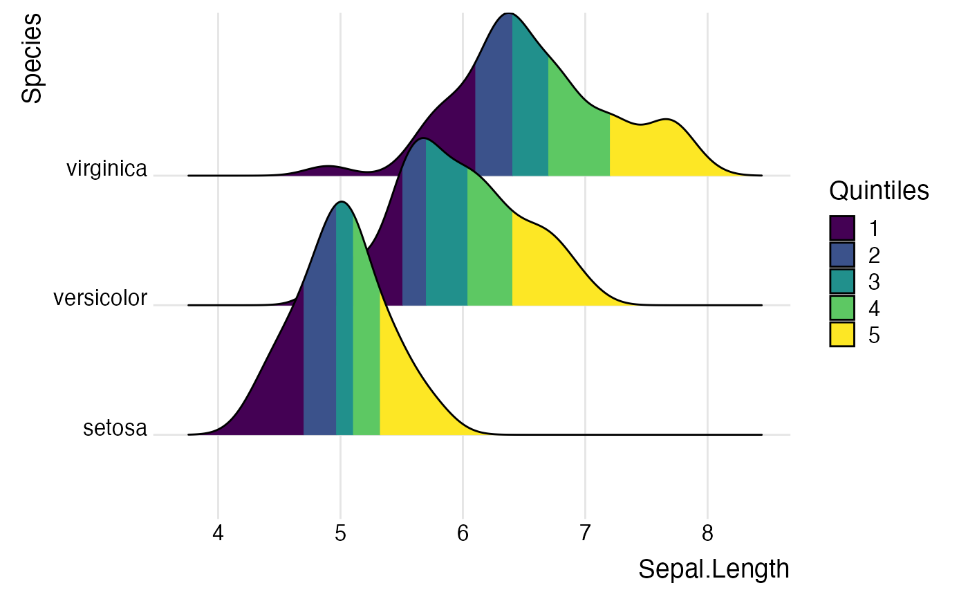
ggplot(iris, aes(x = Sepal.Length, y = Species, fill = factor(stat(quantile)))) +
stat_density_ridges(
geom = "density_ridges_gradient",
calc_ecdf = TRUE,
quantiles = 5
) +
scale_fill_viridis_d(name = "Quintiles") +
theme_ridges()
#> Picking joint bandwidth of 0.181
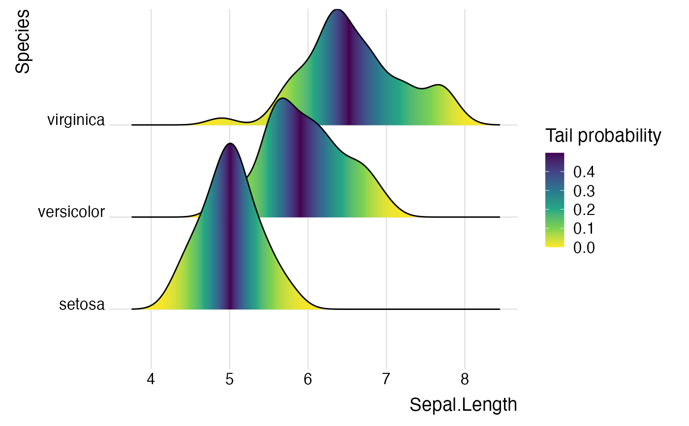
 ggplot(iris,
aes(
x = Sepal.Length, y = Species, fill = 0.5 - abs(0.5-stat(ecdf))
)) +
stat_density_ridges(geom = "density_ridges_gradient", calc_ecdf = TRUE) +
scale_fill_viridis_c(name = "Tail probability", direction = -1) +
theme_ridges()
#> Picking joint bandwidth of 0.181
ggplot(iris,
aes(
x = Sepal.Length, y = Species, fill = 0.5 - abs(0.5-stat(ecdf))
)) +
stat_density_ridges(geom = "density_ridges_gradient", calc_ecdf = TRUE) +
scale_fill_viridis_c(name = "Tail probability", direction = -1) +
theme_ridges()
#> Picking joint bandwidth of 0.181
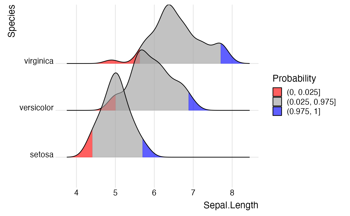
 ggplot(iris,
aes(
x = Sepal.Length, y = Species, fill = factor(stat(quantile))
)) +
stat_density_ridges(
geom = "density_ridges_gradient",
calc_ecdf = TRUE, quantiles = c(0.025, 0.975)
) +
scale_fill_manual(
name = "Probability",
values = c("#FF0000A0", "#A0A0A0A0", "#0000FFA0"),
labels = c("(0, 0.025]", "(0.025, 0.975]", "(0.975, 1]")
) +
theme_ridges()
#> Picking joint bandwidth of 0.181
ggplot(iris,
aes(
x = Sepal.Length, y = Species, fill = factor(stat(quantile))
)) +
stat_density_ridges(
geom = "density_ridges_gradient",
calc_ecdf = TRUE, quantiles = c(0.025, 0.975)
) +
scale_fill_manual(
name = "Probability",
values = c("#FF0000A0", "#A0A0A0A0", "#0000FFA0"),
labels = c("(0, 0.025]", "(0.025, 0.975]", "(0.975, 1]")
) +
theme_ridges()
#> Picking joint bandwidth of 0.181