Corruption and human development
Source:vignettes/corruption_human_development.Rmd
corruption_human_development.RmdFor this example, we will use the following packages.
library(tidyverse)
library(cowplot)    # for theme_minimal_hgrid()
library(colorspace) # for darken()
library(ggrepel)    # for geom_text_repel()
The dataset is provided as practicalgg::corruption. Let’s look at it in table form and in basic scatterplot form.
corrupt <- practicalgg::corruption %>%
  filter(year == 2015) %>%
  na.omit()

corrupt
## # A tibble: 163 x 6
## country region year cpi iso3c hdi
## <chr> <chr> <dbl> <dbl> <chr> <dbl>
## 1 Denmark Europe and Central Asia 2015 91 DNK 0.925
## 2 New Zealand Asia Pacific 2015 91 NZL 0.915
## 3 Finland Europe and Central Asia 2015 90 FIN 0.895
## 4 Sweden Europe and Central Asia 2015 89 SWE 0.913
## 5 Switzerland Europe and Central Asia 2015 86 CHE 0.939
## 6 Norway Europe and Central Asia 2015 88 NOR 0.949
## 7 Singapore Asia Pacific 2015 85 SGP 0.925
## 8 Netherlands Europe and Central Asia 2015 84 NLD 0.924
## 9 Canada Americas 2015 83 CAN 0.92
## 10 Germany Europe and Central Asia 2015 81 DEU 0.926
## # … with 153 more rows
ggplot(corrupt, aes(cpi, hdi, color = region)) +
  geom_point()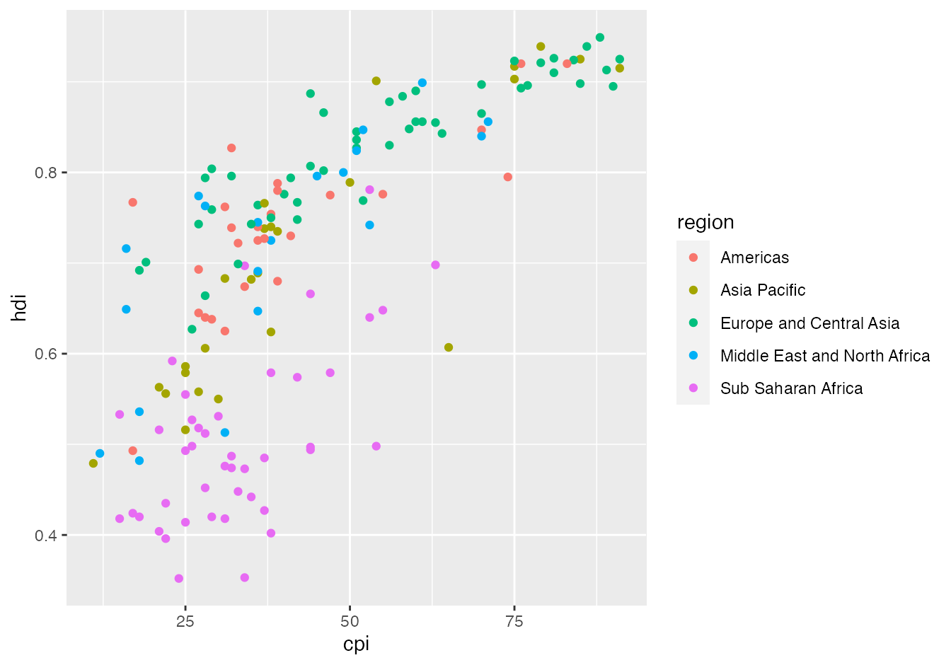
Basic styling: point colors and theme.
# Okabe Ito colors
region_cols <- c("#E69F00", "#56B4E9", "#009E73", "#F0E442", "#0072B2", "#999999")

ggplot(corrupt, aes(cpi, hdi)) +
  geom_point(
    aes(color = region, fill = region),
    size = 2.5, alpha = 0.5, shape = 21
  ) +
  scale_color_manual(
    values = darken(region_cols, 0.3)
  ) +
  scale_fill_manual(
    values = region_cols
  ) +
  theme_minimal_hgrid(12, rel_small = 1) # font size 12 pt throughout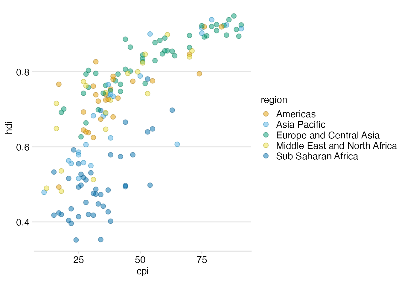
Add smoothing line.
ggplot(corrupt, aes(cpi, hdi)) +
  geom_smooth(
    aes(color = "y ~ log(x)", fill = "y ~ log(x)"),
    method = 'lm', formula = y~log(x), se = FALSE, fullrange = TRUE
  ) +
  geom_point(
    aes(color = region, fill = region),
    size = 2.5, alpha = 0.5, shape = 21
  ) +
  scale_color_manual(
    values = darken(region_cols, 0.3)
  ) +
  scale_fill_manual(
    values = region_cols
  ) +
  theme_minimal_hgrid(12, rel_small = 1)
Set the same scale name for color and fill scale, to force merging of guides.
ggplot(corrupt, aes(cpi, hdi)) +
  geom_smooth(
    aes(color = "y ~ log(x)", fill = "y ~ log(x)"),
    method = 'lm', formula = y~log(x), se = FALSE, fullrange = TRUE
  ) +
  geom_point(
    aes(color = region, fill = region),
    size = 2.5, alpha = 0.5, shape = 21
  ) +
  scale_color_manual(
    name = NULL,
    values = darken(region_cols, 0.3)
  ) +
  scale_fill_manual(
    name = NULL,
    values = region_cols
  ) +
  theme_minimal_hgrid(12, rel_small = 1)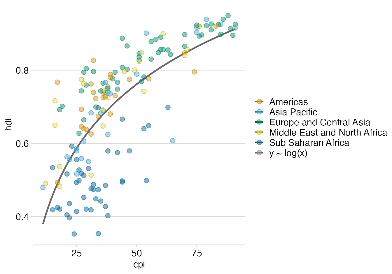
Override legend aesthetics.
ggplot(corrupt, aes(cpi, hdi)) +
  geom_smooth(
    aes(color = "y ~ log(x)", fill = "y ~ log(x)"),
    method = 'lm', formula = y~log(x), se = FALSE, fullrange = TRUE
  ) +
  geom_point(
    aes(color = region, fill = region),
    size = 2.5, alpha = 0.5, shape = 21
  ) +
  scale_color_manual(
    name = NULL,
    values = darken(region_cols, 0.3)
  ) +
  scale_fill_manual(
    name = NULL,
    values = region_cols
  ) +
  guides(
    color = guide_legend(
      override.aes = list(
        linetype = c(rep(0, 5), 1),
        shape = c(rep(21, 5), NA)
      )
    )
  ) +
  theme_minimal_hgrid(12, rel_small = 1)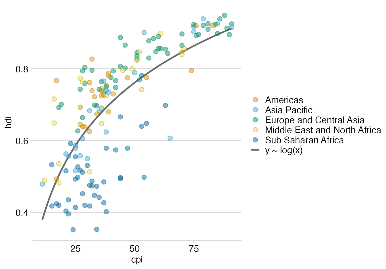
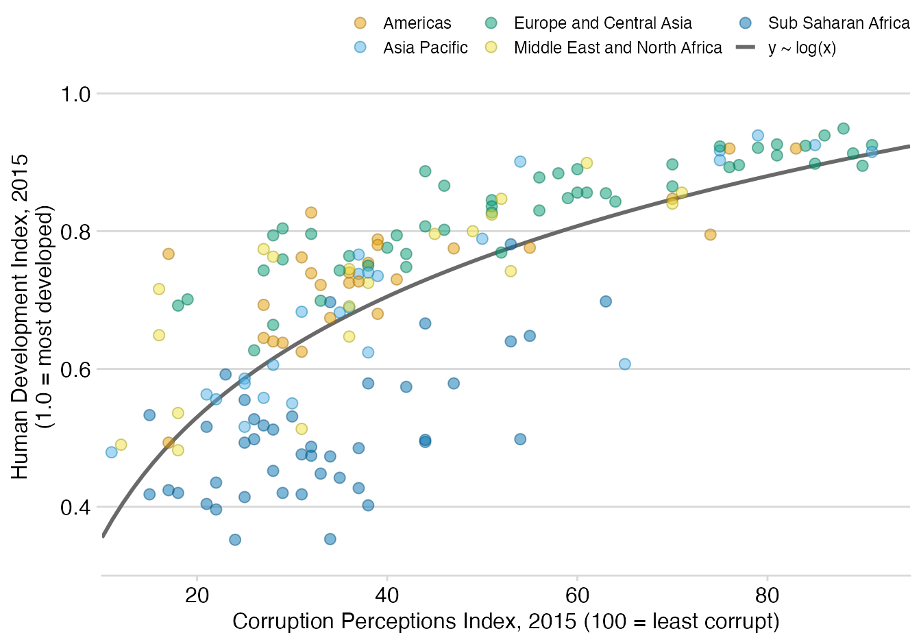
Set x and y scales, move legend on top.
ggplot(corrupt, aes(cpi, hdi)) +
  geom_smooth(
    aes(color = "y ~ log(x)", fill = "y ~ log(x)"),
    method = 'lm', formula = y~log(x), se = FALSE, fullrange = TRUE
  ) +
  geom_point(
    aes(color = region, fill = region),
    size = 2.5, alpha = 0.5, shape = 21
  ) +
  scale_color_manual(
    name = NULL,
    values = darken(region_cols, 0.3)
  ) +
  scale_fill_manual(
    name = NULL,
    values = region_cols
  ) +
  scale_x_continuous(
    name = "Corruption Perceptions Index, 2015 (100 = least corrupt)",
    limits = c(10, 95),
    breaks = c(20, 40, 60, 80, 100),
    expand = c(0, 0)
  ) +
  scale_y_continuous(
    name = "Human Development Index, 2015\n(1.0 = most developed)",
    limits = c(0.3, 1.05),
    breaks = c(0.2, 0.4, 0.6, 0.8, 1.0),
    expand = c(0, 0)
  ) +
  guides(
    color = guide_legend(
      override.aes = list(
        linetype = c(rep(0, 5), 1),
        shape = c(rep(21, 5), NA)
      )
    )
  ) +
  theme_minimal_hgrid(12, rel_small = 1) +
  theme(
    legend.position = "top",
    legend.justification = "right",
    legend.text = element_text(size = 9),
    legend.box.spacing = unit(0, "pt")
  )
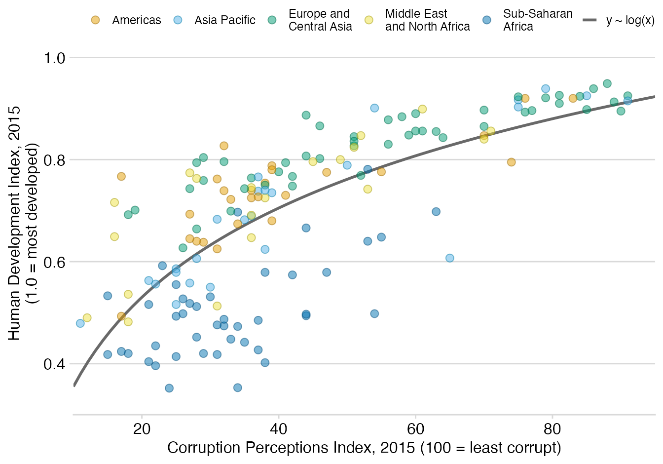
Reformat legend into a single row.
corrupt <- corrupt %>%
  mutate(region = case_when(
    region == "Middle East and North Africa" ~ "Middle East\nand North Africa",
    region == "Europe and Central Asia" ~ "Europe and\nCentral Asia",
    region == "Sub Saharan Africa" ~ "Sub-Saharan\nAfrica",
    TRUE ~ region)
    )

ggplot(corrupt, aes(cpi, hdi)) +
  geom_smooth(
    aes(color = "y ~ log(x)", fill = "y ~ log(x)"),
    method = 'lm', formula = y~log(x), se = FALSE, fullrange = TRUE
  ) +
  geom_point(
    aes(color = region, fill = region),
    size = 2.5, alpha = 0.5, shape = 21
  ) +
  scale_color_manual(
    name = NULL,
    values = darken(region_cols, 0.3)
  ) +
  scale_fill_manual(
    name = NULL,
    values = region_cols
  ) +
  scale_x_continuous(
    name = "Corruption Perceptions Index, 2015 (100 = least corrupt)",
    limits = c(10, 95),
    breaks = c(20, 40, 60, 80, 100),
    expand = c(0, 0)
  ) +
  scale_y_continuous(
    name = "Human Development Index, 2015\n(1.0 = most developed)",
    limits = c(0.3, 1.05),
    breaks = c(0.2, 0.4, 0.6, 0.8, 1.0),
    expand = c(0, 0)
  ) +
  guides(
    color = guide_legend(
      nrow = 1,
      override.aes = list(
        linetype = c(rep(0, 5), 1),
        shape = c(rep(21, 5), NA)
      )
    )
  ) +
  theme_minimal_hgrid(12, rel_small = 1) +
  theme(
    legend.position = "top",
    legend.justification = "right",
    legend.text = element_text(size = 9),
    legend.box.spacing = unit(0, "pt")
  )
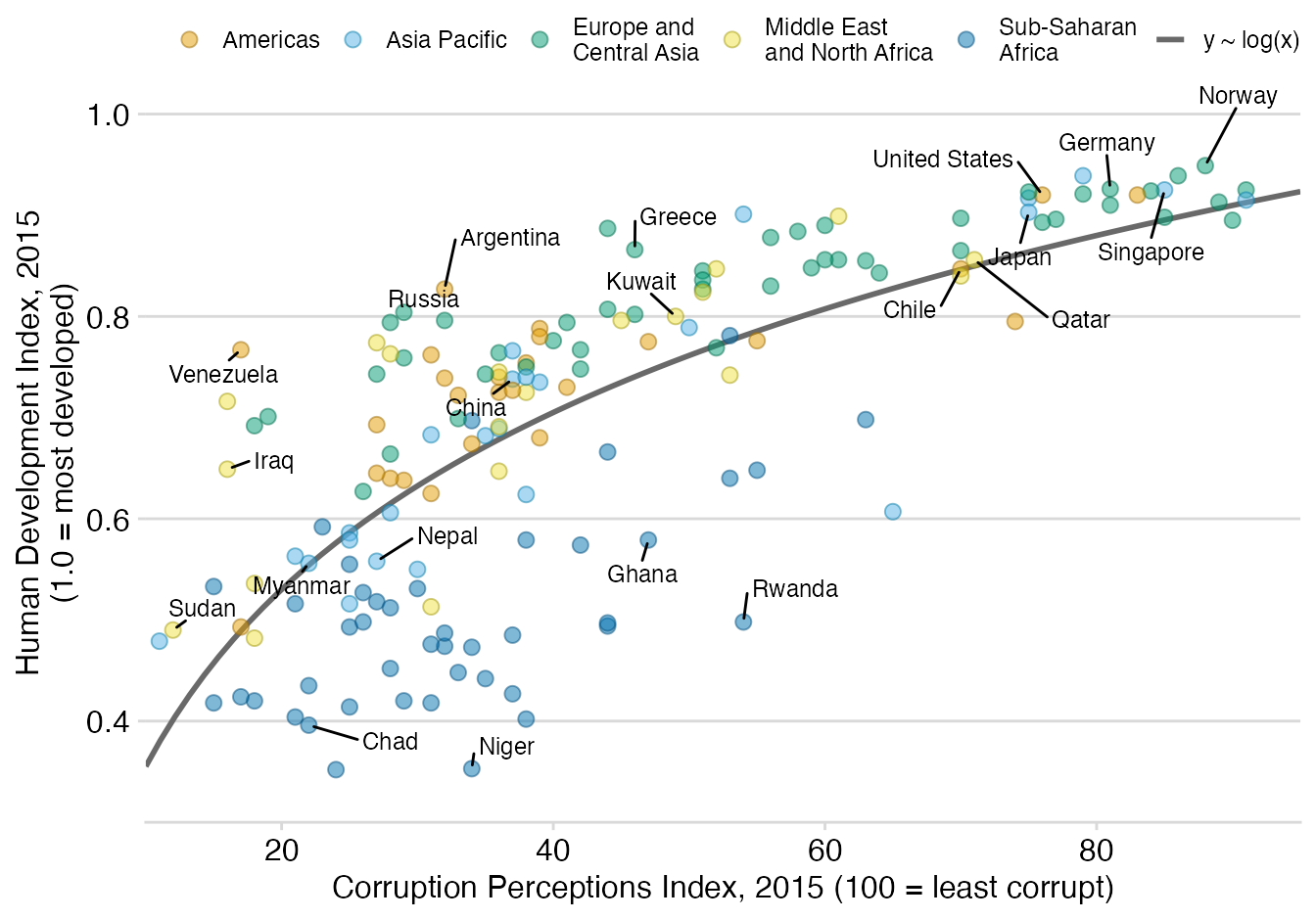
Highlight select countries.
country_highlight <- c("Germany", "Norway", "United States", "Greece", "Singapore", "Rwanda", "Russia", "Venezuela", "Sudan", "Iraq", "Ghana", "Niger", "Chad", "Kuwait", "Qatar", "Myanmar", "Nepal", "Chile", "Argentina", "Japan", "China")

corrupt <- corrupt %>%
  mutate(
    label = ifelse(country %in% country_highlight, country, "")
  )

ggplot(corrupt, aes(cpi, hdi)) +
  geom_smooth(
    aes(color = "y ~ log(x)", fill = "y ~ log(x)"),
    method = 'lm', formula = y~log(x), se = FALSE, fullrange = TRUE
  ) +
  geom_point(
    aes(color = region, fill = region),
    size = 2.5, alpha = 0.5, shape = 21
  ) +
  geom_text_repel(
    aes(label = label),
    color = "black",
    size = 9/.pt, # font size 9 pt
    point.padding = 0.1,
    box.padding = .6,
    min.segment.length = 0,
    max.overlaps = 1000,
    seed = 7654
  ) +
  scale_color_manual(
    name = NULL,
    values = darken(region_cols, 0.3)
  ) +
  scale_fill_manual(
    name = NULL,
    values = region_cols
  ) +
  scale_x_continuous(
    name = "Corruption Perceptions Index, 2015 (100 = least corrupt)",
    limits = c(10, 95),
    breaks = c(20, 40, 60, 80, 100),
    expand = c(0, 0)
  ) +
  scale_y_continuous(
    name = "Human Development Index, 2015\n(1.0 = most developed)",
    limits = c(0.3, 1.05),
    breaks = c(0.2, 0.4, 0.6, 0.8, 1.0),
    expand = c(0, 0)
  ) +
  guides(
    color = guide_legend(
      nrow = 1,
      override.aes = list(
        linetype = c(rep(0, 5), 1),
        shape = c(rep(21, 5), NA)
      )
    )
  ) +
  theme_minimal_hgrid(12, rel_small = 1) +
  theme(
    legend.position = "top",
    legend.justification = "right",
    legend.text = element_text(size = 9),
    legend.box.spacing = unit(0, "pt")
  )